Local Data Tutorial
In this tutorial, rather than running real models and configurations over MIMIC-IV, we’ll work with a set of local, synthetic files distributed with this repository, with the goal being to fully explore the details of this pipeline. This tutorial will consist of both content on this page, running certain scripts on one’s local machine, and some jupyter notebooks. We will walk through the entire pipeline with these local examples and discuss limitations of the pipeline, details of classes, scripts, etc.
We’ll use rootutils to ensure that our notebook is running from the root of the ESGPT repository, to make imports easier.
[1]:
import os
import rootutils

root = rootutils.setup_root(os.path.abspath(''), dotenv=True, pythonpath=True, cwd=True)
Synthetic Data
For this tutorial, we’ll use the three synthetic data files distributed in the sample_data/raw folder in the repository:
[2]:
!ls --color sample_data/raw
admit_vitals.csv labs.csv medications.csv subjects.csv
To see how those files are generated, look at sample_data/generate_synthetic_data.py
These files contain the following data:
subjects.csv
This file contains per-subject data. It has one row per subject, with each row containing a subject identifier (here called “MRN”), a date of birth (”dob”), the subject’s eye color (eye_color), and the subject’s height (”height”):
[3]:
import polars as pl
pl.Config.set_tbl_cols(7)

display(pl.read_csv('sample_data/raw/subjects.csv').head(4))
| MRN | dob | eye_color | height |
|---|---|---|---|
| i64 | str | str | f64 |
| 310243 | "07/28/1981" | "GREEN" | 178.767932 |
| 384198 | "04/15/1985" | "BROWN" | 168.319295 |
| 520533 | "04/15/1979" | "BROWN" | 165.836447 |
| 850710 | "08/08/1970" | "HAZEL" | 159.721833 |
admit_vitals.csv
This file contains dynamic data quantifying both fictional subject hospital admissions, and fictional vitals signs measured for those subjects. Each row of this file records a unique vitals sign measurement for a patient, affiliated with the associated admission listed in the row. This means that admission level information is heavily duplicated within this file, which is a phenomena sometimes observed in real data, and something we’ll need to account for in our pipeline’s setup.
[4]:
display(pl.read_csv('sample_data/raw/admit_vitals.csv').head(4))
| MRN | admit_date | disch_date | department | vitals_date | HR | temp |
|---|---|---|---|---|---|---|
| i64 | str | str | str | str | f64 | f64 |
| 1549363 | "01/04/2010, 06… | "01/14/2010, 11… | "ORTHOPEDIC" | "01/11/2010, 14… | 77.1 | 96.3 |
| 415881 | "02/11/2010, 04… | "02/14/2010, 07… | "ORTHOPEDIC" | "02/11/2010, 10… | 148.5 | 95.6 |
| 42335 | "03/06/2010, 05… | "03/16/2010, 05… | "CARDIAC" | "03/13/2010, 10… | 46.7 | 101.0 |
| 1516810 | "02/11/2010, 23… | "02/22/2010, 23… | "CARDIAC" | "02/12/2010, 16… | 94.2 | 95.2 |
labs.csv
This file contains dynamic data quantifying fictional subject laboratory test measurements. Each row of this file contains a record of a particular lab test measured for a subject. Note that the lab data is not organized into separate columns for each lab; rather each row contains a pair of a lab test name and the associated value; this is what we call in ESGPT a “multivariate regression” column encoding.
[5]:
display(pl.read_csv('sample_data/raw/labs.csv').head(4))
| MRN | timestamp | lab_name | lab_value |
|---|---|---|---|
| i64 | str | str | f64 |
| 1006798 | "10:26:00-2010-… | "SpO2" | 53.0 |
| 739156 | "20:45:44-2010-… | "SpO2" | 51.0 |
| 426870 | "00:25:02-2010-… | "SpO2" | 50.0 |
| 338121 | "17:19:16-2010-… | "GCS" | 1.0 |
Processing Synthetic Data with ESGPT
Now that we see the form of this synthetic data, we can examine how to process it with Event Stream GPT. From the base directory of the ESGPT repository, we can run the following command:
PYTHONPATH=$(pwd):$PYTHONPATH ./scripts/build_dataset.py \
    --config-path="$(pwd)/sample_data/" \
    --config-name=dataset \
    "hydra.searchpath=[$(pwd)/configs]"
Note that this script, like all built-in ESGPT scripts, uses Hydra, a configuration file and experiment run-script library. In hydra, all scripts can take as input a set of composable configuration files which can be overwritten via files or via the command line. If you aren’t already familiar with Hydra, you should read through some of their examples or tutorials to gain some familiarity with their system.
Before we actually run this command, we need to do 2 things:
Decide what we want the command to do, conceptually.
Understand what we’re telling the library to do, via its input arguments.
What do we want to happen?
We can see that our synthetic data has a few different kinds of things happening to these subjects. In the ESGPT data model, we want to organize this data so that we clearly know who our subjects are, quantify when things happen to those subjects, and record in a sparse manner what is happening to those patients. Let’s list a few more specific desiderata:
We should expect our system to quantify those subjects in our synthetic data that meet our inclusion criteria (which we haven’t yet specified).
The system should bucket all interactions for subjects into appropriately defined events, across admissions, discharges, vitals signs, and laboratory tests.
The system should learn appropriate categorical vocabularies, numerical outlier detector models, numerical normalization models, for the various measurements we want to extract (which we haven’t yet specified).
The system should produce “deep-learning friendly” representations of these data.
A quick tangent – what do we mean by “deep-learning friendly” representations of these data? Well, right now, if we were to try to run these data through any deep-learning system for longitudinal data, we’d need to re-format these data such that it is easy to efficiently (ideally \(O(1)\)) retrieve all data corresponding to a single subject in an organized timeseries format that we can then efficiently (meaning in a manner requiring minimal GPU memory) pass into a sequential neural network.
In the current representation, this retrieval process would not be \(O(1)\); instead, if we didn’t modify the data’s organization at all, for each new MRN, we’d need to select from each data file all those rows with that MRN (each selection being an \(O(N)\) operation), and then we would need to subsequently sort all the temporal data by timestamp (another \(O(L\ln(L))\) operation).
Similarly, if we use a naive, dense encoding of the data per measurement for our DL representation, this will be very wasteful in terms of GPU memory, as each record will need to occupy memory proportionate to the total number of possible measurements we could observe in our data (e.g., the total number of lab tests, plus the total number of vitals signs, plus the total number of admission departments, etc.). Instead, a sparse encoding should be used.
These two properties are exactly what we mean by a “deep-learning friendly” representation of the data.
We can see that there are several questions posed by these desiderata that we need to answer, such as:
What are our inclusion criteria?
How should we bucket interactions into events?
What measurements do we want to extract?
How do we want to define “outliers”?
How do we define “appropriate categorical vocabularies”?
How do we want to normalize numerical measurements?
To start us off, let’s use the following answers:
We’ll include all subjects who have at least 3 events, with no other inclusion/exclusion criteria.
We’ll define an “event” to be any interactions happening to a patient within a 1 hour period. We’ll bucket these interactions together starting at the earliest event.
Ideally, we’d like to extract all measurements. As we’ll see, however, due to a limitation in the current version of ESGPT, we’ll extract all measurements except for the patient’s height. In particular, we’ll extract the occurrence of admissions, discharges, vitals signs, and laboratory tests, as well as the subject’s age, eye color, admission department, the values recorded for HR and temperature, and all lab test values.
We’ll use a very simple outlier model, that excludes numerical data as outliers if their values exceed 1.5 standard deviations from the mean. This is an extremely aggressive cutoff only suitable for this synthetic data setting.
We’ll keep any categorical observation as a vocabulary element if it occurs at least 5 times.
We’ll normalize our numerical observations to have zero mean and unit variance.
Telling the pipeline what to do: input config
Now that we have some basic idea of what we want the pipeline to do, let’s examine the input configuration file that we pass to the dataset script:
[6]:
!cat sample_data/dataset.yaml
defaults:
  - dataset_base
  - _self_

# So that it can be run multiple times without issue.
do_overwrite: True

cohort_name: "sample"
subject_id_col: "MRN"
raw_data_dir: "./sample_data/raw/"
save_dir: "./sample_data/processed/${cohort_name}"

DL_chunk_size: null

inputs:
  subjects:
    input_df: "${raw_data_dir}/subjects.csv"
  admissions:
    input_df: "${raw_data_dir}/admit_vitals.csv"
    start_ts_col: "admit_date"
    end_ts_col: "disch_date"
    ts_format: "%m/%d/%Y, %H:%M:%S"
    event_type: ["OUTPATIENT_VISIT", "ADMISSION", "DISCHARGE"]
  vitals:
    input_df: "${raw_data_dir}/admit_vitals.csv"
    ts_col: "vitals_date"
    ts_format: "%m/%d/%Y, %H:%M:%S"
  labs:
    input_df: "${raw_data_dir}/labs.csv"
    ts_col: "timestamp"
    ts_format: "%H:%M:%S-%Y-%m-%d"

measurements:
  static:
    single_label_classification:
      subjects: ["eye_color"]
  functional_time_dependent:
    age:
      functor: AgeFunctor
      necessary_static_measurements: { "dob": ["timestamp", "%m/%d/%Y"] }
      kwargs: { dob_col: "dob" }
  dynamic:
    multi_label_classification:
      admissions: ["department"]
    univariate_regression:
      vitals: ["HR", "temp"]
    multivariate_regression:
      labs: [["lab_name", "lab_value"]]

outlier_detector_config:
  stddev_cutoff: 1.5
min_valid_vocab_element_observations: 5
min_valid_column_observations: 5
min_true_float_frequency: 0.1
min_unique_numerical_observations: 20
min_events_per_subject: 3
agg_by_time_scale: "1h"
There are a number of sections in this file. Firstly, the first three lines ensure this config builds on the defaults provided with the ESGPT library, via Hydra’s normal mechanisms. If you aren’t familiar with this syntax, check out the Hydra documentation.
Next, there is a section defining some overarching variables and a section defining our input sources. We can see this section details the paths to each of our input files as well as the formatting used for (most of) the timestamps within these files. Note that this section makes use of Hydra/OmegaConf’s Interpolations to simplify the specification of the file paths used.
Warning: Two parameters in this section are required: subject_id_col, and cohort_name. This will be explored in more detail later in this tutorial.
Next, we have a section defining the various measurements we’ll exctract in this dataset. We can see we specify each of the measurements we discussed above: 1. eye_color is extracted as a static, single_label_classification measure. 2. age is extracted as a functional_time_dependent measure, leveraging the date-of-birth column dob. Note that this is where we define the timestamp format for the ``dob`` column, as it is a timestamp formatted static column! 3.
department is extracted as a dynamic, multi_label_classification measure. 4. HR, and temp are extracted as dynamic, univariate_regression measures. 5. lab_name and lab_value are extracted as a single dynamic, multivariate_regression measure.
Note that the terms static, functional_time_dependent, & dynamic and single_label_classification, multi_label_classification, univariate_regression, and multivariate_regression, are defined enumerations in the EventStream.data.config sub-module, and dictate where measurements are stored and how they are pre-processed.
Finally, we have the remaining set of parameters, which define our inclusion-exclusion criteria (by specifying min_events_per_subject), our outlier and normalizer model configuration parameters (normalization being omitted here as what we want is the default value), our filtering thresholds for vocabulary elements, and the aggregation time-scale for events.
What else could we have specified?
To better understand the structure of this input specification, let’s explore this input configuration file in a bit more detail. To start with, let’s look at what the default, base config contains (the config we inherit from in the defaults list):
[7]:
!cat configs/dataset_base.yaml
defaults:
  - outlier_detector_config: stddev_cutoff
  - normalizer_config: standard_scaler
  - _self_

cohort_name: ???
save_dir: ${oc.env:PROJECT_DIR}/data/${cohort_name}
subject_id_col: ???
seed: 1
split: [0.8, 0.1]
do_overwrite: False
DL_chunk_size: 20000
min_valid_vocab_element_observations: 25
min_valid_column_observations: 50
min_true_float_frequency: 0.1
min_unique_numerical_observations: 25
min_events_per_subject: 20
agg_by_time_scale: null

hydra:
  job:
    name: build_${cohort_name}
  run:
    dir: ${save_dir}/.logs
  sweep:
    dir: ${save_dir}/.logs
We can see there are some parameters we’re familiar with and some we’re not. Firstly, we can see that this default base config marks cohort_name and subject_id_col with ???. This is the OmegaConf provided value to represent a value that needs to be overwritten in downstream usage. This is why those two parameters are mandatory. This config also has variables for the seed, split size, and some hydra-internal parameters. Further, it points to two further default configs for the
outlier detector and normalizer:
[8]:
!cat configs/outlier_detector_config/stddev_cutoff.yaml
cls: stddev_cutoff
stddev_cutoff: 5.0
[9]:
!cat configs/normalizer_config/standard_scaler.yaml
cls: standard_scaler
These are both quite simple, but show how the final config will be constructed from these values.
One thing that is notably missing from this broader structure is any notion of included inputs or measurements sections. To understand how we can further specify our config, we need to understand how we could modify those sections as well.
Inputs
This section allows us to specify which input data frames should be read, and from where. The inputs: option should be an object whose keys are the names of input sources and whose values are configuration for those inputs. Currently, two input formats are possible:
The
input_dfformat, which is used in this synthetic example. This format has an input configuration that contains theinput_df:key whose value is a file path pointing to acsvorparquetdata-frame file on disk that contains that input source’s data. For example:
admissions:
  input_df: "${raw_data_dir}/admit_vitals.csv"
  start_ts_col: "admit_date"
  end_ts_col: "disch_date"
  ts_format: "%m/%d/%Y, %H:%M:%S"
  event_type: ["OUTPATIENT_VISIT", "ADMISSION", "DISCHARGE"]
The
queryformat, which is used in the MIMIC-IV tutorial. In this format, you must specify aqueryparameter. This parameter can either be a string query or a list of string queries, in which case you must specify a globalconnection_uriparameter detailing the URI of the database to which you wish to query (In the connector-x format), or a dictionary, with keys and values specifying parameters of the`EventStream.data.dataset_polars.Query<>`__ object. For example:
patients:
  query: |-
    SELECT subject_id, gender, to_date((anchor_year-anchor_age)::CHAR(4), 'YYYY') AS year_of_birth
    FROM mimiciv_hosp.patients
    WHERE subject_id IN (
      SELECT long_icu.subject_id FROM (
        (
          SELECT subject_id FROM mimiciv_icu.icustays WHERE los > ${min_los}
        ) AS long_icu INNER JOIN (
          SELECT subject_id
          FROM mimiciv_hosp.admissions
          GROUP BY subject_id
          HAVING COUNT(*) > ${min_admissions}
        ) AS many_admissions
        ON long_icu.subject_id = many_admissions.subject_id
      )
    )
  must_have: ["gender", "year_of_birth"]
Each input can also have a number of other keys and values, including:
Timestamp & Event-type Specification.
For non-static data sources, the keys ts_col or start_ts_col and end_ts_col specify the name of the column (or columns) containing the timestamp for the event, and ts_format the format of that timestamp. ts_col is used for data-sources where each row represents one event, and start_/end_ts_col for data-sources where each row specifies a range in time. For example, in our synthetic config,
admissions:
    input_df: "${raw_data_dir}/admit_vitals.csv"
    start_ts_col: "admit_date"
    end_ts_col: "disch_date"
    ts_format: "%m/%d/%Y, %H:%M:%S"
    event_type: ["OUTPATIENT_VISIT", "ADMISSION", "DISCHARGE"]
specifies a range event, where the start timestamp is stored in admit_date and the end timestamp in disch_date, formatted as "%m/%d/%Y, %H:%M:%S". In contrast,
labs:
    input_df: "${raw_data_dir}/labs.csv"
    ts_col: "timestamp"
    ts_format: "%H:%M:%S-%Y-%m-%d"
captures data where each row is a single-timepoint event, with timestamp stored in "%H:%M:%S-%Y-%m-%d" format in column timestamp.
You can also explicitly set the type of each event. Events’ types in ESGPT are categorical variables defined by the user that are used to dictate any intra-event causal dependency graphs in downstream models, can be used to help define downstream tasks, and are otherwise used to analyze and describe data. When using the pre-defined build dataset script, they can either be explicitly set or are automatically inferred from the name of the input block. For example, in the examples given above, the
labs: block produces an input source with the event type LAB (the singular, upper-cased inflection of the name of the block, 'labs'), and admissions (being a range event) produces events of type 'OUTPATIENT_VISIT' when admit_date == disch_date and 'ADMISSION' on admit_date and 'DISCHARGE' on disch_date. For range events, the default event types are defined to be *_EQ, *_START, and *_END, where * is the singular, upper-cased inflection of
the input block name.
Event types can also be defined to be column dependent. For example, in this config example (which is not part of our current synthetic example config), we see that event types are defined to take on the value of the column 'visit_occurrence_concept_name' for the case that the start and end times are the same and for start events, but the static 'Drug Stop' for end events.
drugs:
    input_df: "${raw_data_dir}/drug.parquet"
    start_ts_col: "drug_exposure_start_datetime"
    end_ts_col: ["drug_exposure_end_datetime", "verbatim_end_date"]
    event_type: ["COL:visit_occurrence_concept_name", "COL:visit_occurrence_concept_name", "Drug Stop"]
    start_columns: {"standard_concept_name": "drug", "drug_type_concept_name": "drug_type"}
    end_columns:
        standard_concept_name: drug
        drug_type_concept_name: drug_type
        stop_reason: drug_stop_reason
Filtering
You can also specify a simple filter used for a given input source. For example, in the patients block in the MIMIC-IV example, we specify that valid rows must have 'gender' and 'year_of_birth' defined and non-null. This is another way to enforce cohort inclusion/exclusion criteria. The filter object can either be a list of strings, in which case those columns must have non-null values, or a dictionary from column names to either the boolean True (indicating the column must be
present and non-null) or lists of allowable values for that column.
Measurement columns to extract
You can also specify which measurements should be extracted to associate with a given input data source. Largely, this information will be determined automatically based on the measurements section of the config; however, it can be specified explicitly as well. The most common case this would be done is to differentiate different measurements to associate with start and end events for range events or to re-name measurements from their input column names to new names for internal use
(this can be done not only for cosmetic reasons, but so as to unify or disentangle measurements across different input files). For example, in the drugs: example shown above, the columns standard_concept_name and drug_type_concept_name are both used for both start and end events, and are renamed to 'drug', and 'drug_type' in both cases, whereas stop_reason is used only for end events (and is renamed to drug_stop_reason). ##### Measurements Section The
measurements: block lists all the actual measurements that should be extracted from those input sources, broken down into categories based on their temporality and modality (see EventStream.data.types.TemporalityType and EventStream.data.types.DataModality, respectively).
The only non-standard portion of this block corresponds to the functional_time_dependent block, which specifies measurements whose values are not stored in the raw input data by default, but are instead computable dynamically given per-subject static data and the timestamps of other events that occur in the data. A good example is a subject’s age, which is included in our synthetic configuration. Given a subject’s date-of-birth and the timestamp of any other event, we can dynamically
compute the subject’s age as of that event, which is exactly what the EventStream.data.time_dependent_functor.AgeFunctor does.
The structure of this config section is
functional_time_dependent:
  output_measurement_name:
      functor: ??? # The functor that is used for this measurement. Must be in `EventStream.data.config.MeasurementConfig.FUNCTORS`
      necessary_static_measurements: { "static_measurement_column": ??? } # column name: column formatting info
      kwargs: { kwarg: kwval } # Keyword args to pass to functor constructor.
Currently, only `AgeFunctor <>`__ and [TimeOfDayFunctor] are pre-defined and supported, but this can be extended by the user by directly adding new functors to the `EventStream.data.config.MeasurementConfig <>`__ object.
Running the Command
Now that we understand the setup a bit better, let’s run the actual command:
PYTHONPATH=$(pwd):$PYTHONPATH ./scripts/build_dataset.py \
    --config-path="$(pwd)/sample_data/" \
    --config-name=dataset \
    "hydra.searchpath=[$(pwd)/configs]"
To make this notebook self sufficient, we’ll run it here via the `subprocess <>`__ module:
[10]:
import subprocess

command = """\
PYTHONPATH=$(pwd):$PYTHONPATH ./scripts/build_dataset.py \
 --config-path="$(pwd)/sample_data/" \
 --config-name=dataset \
 "hydra.searchpath=[$(pwd)/configs]" """

command_out = subprocess.run(command, shell=True, capture_output=True)
print(command_out.stdout.decode())

if command_out.returncode == 1:
    print("Command Errored!")

print(command_out.stderr.decode())
Empty new events dataframe of type OUTPATIENT_VISIT!
You should see as output the printed line Empty new events dataframe of type OUTPATIENT_VISIT!, but otherwise nothing. Before we proceed further, let’s break down what this process has done, and how it could do things differently.
Firstly, let’s take a look at what is produced in the output folder itself.
[11]:
!du -sh sample_data/processed/sample/
2.3M sample_data/processed/sample/
[12]:
!ls --color -R sample_data/processed/sample
sample_data/processed/sample:
config.json                      inferred_measurement_configs.json
DL_reps                          inferred_measurement_metadata
dynamic_measurements_df.parquet  input_schema.json
E.pkl                            subjects_df.parquet
events_df.parquet                vocabulary_config.json
hydra_config.yaml

sample_data/processed/sample/DL_reps:
held_out_0.parquet  train_0.parquet  tuning_0.parquet

sample_data/processed/sample/inferred_measurement_metadata:
age.csv  HR.csv  lab_name.csv  temp.csv
Now, let’s walk through what happens when we run this script, step-by-step, and how each of the files listed above are produced.
Step 1: Config Parsing
First, the script parses our input config file into a slightly refined structured form, then passes that as input to the EventStream.data.dataset_polars.Dataset constructor.
To see what this process looks like, we can inspect one portion of the output of the overall script, which we can find in the `sample_data/processed/sample <>`__ directory; in particular, the input_schema.json file.
Note that the sample_data/processed/sample directory is the save_dir key in our dataset.yaml configuration file.
[13]:
!cat sample_data/processed/sample/input_schema.json | python -m json.tool
{
    "static": {
        "input_df": "./sample_data/raw//subjects.csv",
        "type": "static",
        "event_type": null,
        "subject_id_col": "MRN",
        "ts_col": null,
        "start_ts_col": null,
        "end_ts_col": null,
        "ts_format": null,
        "start_ts_format": null,
        "end_ts_format": null,
        "data_schema": [
            {
                "eye_color": "categorical",
                "dob": [
                    "dob",
                    [
                        "timestamp",
                        "%m/%d/%Y"
                    ]
                ]
            }
        ],
        "start_data_schema": null,
        "end_data_schema": null,
        "must_have": []
    },
    "dynamic": [
        {
            "input_df": "./sample_data/raw//admit_vitals.csv",
            "type": "range",
            "event_type": [
                "OUTPATIENT_VISIT",
                "ADMISSION",
                "DISCHARGE"
            ],
            "subject_id_col": "MRN",
            "ts_col": null,
            "start_ts_col": "admit_date",
            "end_ts_col": "disch_date",
            "ts_format": null,
            "start_ts_format": "%m/%d/%Y, %H:%M:%S",
            "end_ts_format": "%m/%d/%Y, %H:%M:%S",
            "data_schema": [
                {
                    "department": "categorical"
                }
            ],
            "start_data_schema": [
                {
                    "department": "categorical"
                }
            ],
            "end_data_schema": [
                {
                    "department": "categorical"
                }
            ],
            "must_have": []
        },
        {
            "input_df": "./sample_data/raw//admit_vitals.csv",
            "type": "event",
            "event_type": "VITAL",
            "subject_id_col": "MRN",
            "ts_col": "vitals_date",
            "start_ts_col": null,
            "end_ts_col": null,
            "ts_format": "%m/%d/%Y, %H:%M:%S",
            "start_ts_format": null,
            "end_ts_format": null,
            "data_schema": [
                {
                    "HR": "float",
                    "temp": "float"
                }
            ],
            "start_data_schema": null,
            "end_data_schema": null,
            "must_have": []
        },
        {
            "input_df": "./sample_data/raw//labs.csv",
            "type": "event",
            "event_type": "LAB",
            "subject_id_col": "MRN",
            "ts_col": "timestamp",
            "start_ts_col": null,
            "end_ts_col": null,
            "ts_format": "%H:%M:%S-%Y-%m-%d",
            "start_ts_format": null,
            "end_ts_format": null,
            "data_schema": [
                {
                    "lab_name": "categorical",
                    "lab_value": "float"
                }
            ],
            "start_data_schema": null,
            "end_data_schema": null,
            "must_have": []
        }
    ]
}
This object, stored in JSON format, is an instance of the EventStream.data.config.DatasetSchema object; interested readers can read more about it’s specific formatting requirements there. We can see that this contains much of the same information as was in the initial dataset.yaml config shown above, now with some additional data added as well, such as recognizing that the "lab_name" column should be read in as a categorical type and "lab_value" as a float type.
Beyond the input data schema, the model also writes out the ESGPT’s input overall config object to disk, which stores information about which measurements the pipeline is instructed to extract. That object is stored in config.json:
[14]:
!cat sample_data/processed/sample/config.json | python -m json.tool
{
    "measurement_configs": {
        "eye_color": {
            "name": "eye_color",
            "temporality": "static",
            "modality": "single_label_classification",
            "observation_rate_over_cases": null,
            "observation_rate_per_case": null,
            "functor": null,
            "vocabulary": null,
            "values_column": null,
            "_measurement_metadata": null,
            "modifiers": null
        },
        "department": {
            "name": "department",
            "temporality": "dynamic",
            "modality": "multi_label_classification",
            "observation_rate_over_cases": null,
            "observation_rate_per_case": null,
            "functor": null,
            "vocabulary": null,
            "values_column": null,
            "_measurement_metadata": null,
            "modifiers": null
        },
        "HR": {
            "name": "HR",
            "temporality": "dynamic",
            "modality": "univariate_regression",
            "observation_rate_over_cases": null,
            "observation_rate_per_case": null,
            "functor": null,
            "vocabulary": null,
            "values_column": null,
            "_measurement_metadata": null,
            "modifiers": null
        },
        "temp": {
            "name": "temp",
            "temporality": "dynamic",
            "modality": "univariate_regression",
            "observation_rate_over_cases": null,
            "observation_rate_per_case": null,
            "functor": null,
            "vocabulary": null,
            "values_column": null,
            "_measurement_metadata": null,
            "modifiers": null
        },
        "lab_name": {
            "name": "lab_name",
            "temporality": "dynamic",
            "modality": "multivariate_regression",
            "observation_rate_over_cases": null,
            "observation_rate_per_case": null,
            "functor": null,
            "vocabulary": null,
            "values_column": "lab_value",
            "_measurement_metadata": null,
            "modifiers": null
        },
        "age": {
            "name": "age",
            "temporality": "functional_time_dependent",
            "modality": "univariate_regression",
            "observation_rate_over_cases": null,
            "observation_rate_per_case": null,
            "functor": {
                "class": "AgeFunctor",
                "params": {
                    "dob_col": "dob"
                }
            },
            "vocabulary": null,
            "values_column": null,
            "_measurement_metadata": null,
            "modifiers": null
        }
    },
    "min_events_per_subject": 3,
    "agg_by_time_scale": "1h",
    "min_valid_column_observations": 5,
    "min_valid_vocab_element_observations": 5,
    "min_true_float_frequency": 0.1,
    "min_unique_numerical_observations": 20,
    "outlier_detector_config": {
        "cls": "stddev_cutoff",
        "stddev_cutoff": 1.5
    },
    "normalizer_config": {
        "cls": "standard_scaler"
    },
    "save_dir": "/home/mmd/Projects/EventStreamGPT/sample_data/processed/sample"
}
Again, much of this information is simply a more verbose re-arrangement of the data specified in dataset.yaml. Notably, no information about the measurements has yet been filled in from the data, though it will eventually be added.
This config structure illustrates a capability of the pipeline outside of the traditional input script format; namely, if one constructs the full config manually, one can pre-specify various measurement specific values (such as vocabulary, normalization parameters, etc.) to be used over what would be inferred from the data.
There is also the full, expanded hydra config stored in hydra_config.yaml, which can help aid in reproducibility.
The final input to the constructor of the EventStream.data.dataset_polars.Dataset class can be seen in the documentation for its base class, EventStream.data.dataset_base.DatasetBase and takeas input:
A
configobject (like that shown in JSON form above.Either the
subjects_df,events_df, anddynamic_measurements_dfdataframes directly or aninput_schemaEventStream.data.config.DatasetSchemaobject which is shown ininput_schema.jsonabove, which is used to construct the three dataframes from source. Currently, the immediate extraction output is not written to disk at all, so we can’t directly inspect thesubjects_df,events_df, anddynamic_measurements_dfthat result from ourinput_schema, but we can see their relative structure from the final, pre-processed dataframes which are written to disk, which we’ll explore next.
Step 2: Data reading and pre-processing
After normalizing the input configs, the pipeline next extracts the data from source and performs pre-processing on these dataframes. This pre-processing encompasses several steps, including:
Minimizing data types to minimizing memory/disk footprint.
Splitting data into train, hyperparameter tuning, and held out test sets.
Identifying categorical variable vocabularies.
Converting appropriate numerical variables to categorical.
Fitting numerical outlier detectors and normalizers.
Normalizing numerical data, removing outliers and infrequent vocabulary elements, and writing out processed
subjects_df,events_df, anddynamic_measurements_dfparquet files.
Pre-processed Data Frames
After this process is complete, we gain the following three files. Note that we’ll inspect the files manually here, but you can also load the dataset object and inspect them that way, which we’ll do below.
[15]:
!ls --color sample_data/processed/sample/*_df.parquet
sample_data/processed/sample/dynamic_measurements_df.parquet
sample_data/processed/sample/events_df.parquet
sample_data/processed/sample/subjects_df.parquet
[16]:
# We use polars to look at these parquet files:
import polars as pl
pl.Config.set_tbl_cols(7)

display(pl.scan_parquet('sample_data/processed/sample/subjects_df.parquet').head(4).collect())
| subject_id | MRN | eye_color | dob |
|---|---|---|---|
| u8 | cat | cat | datetime[μs] |
| 0 | "310243" | "GREEN" | 1981-07-28 00:00:00 |
| 1 | "384198" | "BROWN" | 1985-04-15 00:00:00 |
| 2 | "520533" | "BROWN" | 1979-04-15 00:00:00 |
| 3 | "850710" | "HAZEL" | 1970-08-08 00:00:00 |
The subjects dataframe subjects_df contains subject IDs (which have been re-named and normalized to occupy the minimal possible uint type (here uint8), and contains a categorical eye_color column for our static measurement, but height has been dropped as it wasn’t included in our config.
[17]:
display(pl.scan_parquet('sample_data/processed/sample/events_df.parquet').head(4).collect())
| event_id | subject_id | timestamp | event_type | age | age_is_inlier |
|---|---|---|---|---|---|
| u32 | u8 | datetime[μs] | cat | f64 | bool |
| 0 | 0 | 2010-06-24 13:23:00 | "ADMISSION&VITA… | -0.463849 | true |
| 1 | 0 | 2010-06-24 14:23:00 | "VITAL&LAB" | -0.463823 | true |
| 2 | 0 | 2010-06-24 15:23:00 | "VITAL&LAB" | -0.463796 | true |
| 3 | 0 | 2010-06-24 16:23:00 | "VITAL&LAB" | -0.46377 | true |
The events dataframe events_df contains event IDs, subject IDs, timestamps, event types, and our only functional time dependent measurement, age, in normalized form, alongside an inlier/outlier indicator column. We can also see several other properties: 1. That these data are sorted, first by subject_id then by event_id (equivalently, by timestamp). 2. That event timestamps are separated by precisely 1 hour, which was our input aggregation window. 3. That event types have
been aggregated into merged categories during aggregation. E.g., event 1 with event type VITAL&LAB reflects that events of type VITAL and LAB have been merged together. This is to ensure that no subject has two distinct events at the same timestamp.
[18]:
df = pl.scan_parquet('sample_data/processed/sample/dynamic_measurements_df.parquet')
print("Dynamic Measurement Columns:\n  * " + '\n  * '.join(df.columns))
display(df.head(4).collect())
Dynamic Measurement Columns:
  * measurement_id
  * department
  * HR
  * temp
  * lab_name
  * lab_value
  * event_id
  * HR_is_inlier
  * temp_is_inlier
  * lab_name_is_inlier
| measurement_id | department | HR | … | HR_is_inlier | temp_is_inlier | lab_name_is_inlier |
|---|---|---|---|---|---|---|
| u32 | cat | f64 | … | bool | bool | bool |
| 0 | "CARDIAC" | null | … | null | null | null |
| 1 | "PULMONARY" | null | … | null | null | null |
| 2 | "CARDIAC" | null | … | null | null | null |
| 3 | "PULMONARY" | null | … | null | null | null |
The dynamic measurements dataframe dynamic_measurements_df has an ID column, an event_id linking column, and then all our measurements, recorded with missingness.
Fit Measurement Properties
In all of these dataframes, we can see the outputs from our learned vocabularies, outlier detector models, and normalizer models. How can we determine what fit parameters were used to make those distinctions? These data are stored in the inferred_measurement_metadata objects. The overall container is stored in inferred_measurement_configs.json, which contains an object linking measurement names to overall configs:
[19]:
!cat sample_data/processed/sample/inferred_measurement_configs.json | python -m json.tool
{
    "eye_color": {
        "name": "eye_color",
        "temporality": "static",
        "modality": "single_label_classification",
        "observation_rate_over_cases": 1.0,
        "observation_rate_per_case": 1.0,
        "functor": null,
        "vocabulary": {
            "vocabulary": [
                "UNK",
                "BROWN",
                "BLUE",
                "HAZEL",
                "GREEN"
            ],
            "obs_frequencies": [
                0.0,
                0.5125,
                0.2125,
                0.175,
                0.1
            ]
        },
        "values_column": null,
        "_measurement_metadata": null,
        "modifiers": null
    },
    "department": {
        "name": "department",
        "temporality": "dynamic",
        "modality": "multi_label_classification",
        "observation_rate_over_cases": 0.012158770003137746,
        "observation_rate_per_case": 1.0,
        "functor": null,
        "vocabulary": {
            "vocabulary": [
                "UNK",
                "PULMONARY",
                "CARDIAC",
                "ORTHOPEDIC"
            ],
            "obs_frequencies": [
                0.0,
                0.3870967741935484,
                0.36451612903225805,
                0.24838709677419354
            ]
        },
        "values_column": null,
        "_measurement_metadata": null,
        "modifiers": null
    },
    "HR": {
        "name": "HR",
        "temporality": "dynamic",
        "modality": "univariate_regression",
        "observation_rate_over_cases": 0.7112880451835583,
        "observation_rate_per_case": 1.7473945409429281,
        "functor": null,
        "vocabulary": null,
        "values_column": null,
        "_measurement_metadata": [
            "/home/mmd/Projects/EventStreamGPT/sample_data/processed/sample",
            "inferred_measurement_metadata/HR.csv"
        ],
        "modifiers": null
    },
    "temp": {
        "name": "temp",
        "temporality": "dynamic",
        "modality": "univariate_regression",
        "observation_rate_over_cases": 0.7112880451835583,
        "observation_rate_per_case": 1.7473945409429281,
        "functor": null,
        "vocabulary": null,
        "values_column": null,
        "_measurement_metadata": [
            "/home/mmd/Projects/EventStreamGPT/sample_data/processed/sample",
            "inferred_measurement_metadata/temp.csv"
        ],
        "modifiers": null
    },
    "lab_name": {
        "name": "lab_name",
        "temporality": "dynamic",
        "modality": "multivariate_regression",
        "observation_rate_over_cases": 0.9564637590210229,
        "observation_rate_per_case": 1.8052161076027229,
        "functor": null,
        "vocabulary": {
            "vocabulary": [
                "UNK",
                "SpO2",
                "potassium",
                "creatinine",
                "SOFA__EQ_1",
                "SOFA__EQ_2",
                "GCS__EQ_1",
                "SOFA__EQ_3",
                "GCS__EQ_4",
                "GCS__EQ_3",
                "GCS__EQ_2",
                "SOFA__EQ_4",
                "GCS__EQ_5",
                "GCS__EQ_6",
                "GCS__EQ_8",
                "GCS__EQ_7",
                "GCS__EQ_11",
                "GCS__EQ_9",
                "GCS__EQ_10",
                "GCS__EQ_12",
                "GCS__EQ_15",
                "GCS__EQ_14",
                "GCS__EQ_13"
            ],
            "obs_frequencies": [
                0.0,
                0.8298577983735405,
                0.04302394257416746,
                0.03820816864295125,
                0.02959883694516378,
                0.012743628185907047,
                0.010403888964608605,
                0.005315524056153742,
                0.003679978192721821,
                0.0033165235564036164,
                0.003043932579164963,
                0.002930353005315524,
                0.002748625687156422,
                0.002203443732679115,
                0.0021352959883694515,
                0.0020898641588296763,
                0.001680977692971696,
                0.0016582617782018082,
                0.0016582617782018082,
                0.0010676479941847258,
                0.0009086365907955114,
                0.0008632047612557358,
                0.0008632047612557358
            ]
        },
        "values_column": "lab_value",
        "_measurement_metadata": [
            "/home/mmd/Projects/EventStreamGPT/sample_data/processed/sample",
            "inferred_measurement_metadata/lab_name.csv"
        ],
        "modifiers": null
    },
    "age": {
        "name": "age",
        "temporality": "functional_time_dependent",
        "modality": "univariate_regression",
        "observation_rate_over_cases": 1.0,
        "observation_rate_per_case": 1.0,
        "functor": {
            "class": "AgeFunctor",
            "params": {
                "dob_col": "dob"
            }
        },
        "vocabulary": null,
        "values_column": null,
        "_measurement_metadata": [
            "/home/mmd/Projects/EventStreamGPT/sample_data/processed/sample",
            "inferred_measurement_metadata/age.csv"
        ],
        "modifiers": null
    }
}
We can see that these objects contain the full vocabularies learned, as well as (for numerical measurements) internal links to further measurement metadata csv files. These csv files contain more detailed statistics for numerical data, such as outlier detector and normalizer models. Let’s inspect two of these, one for the multivariate_regression measurement lab_name and one for the univariate_regression measurement age:
[20]:
display(pl.read_csv('sample_data/processed/sample/inferred_measurement_metadata/lab_name.csv').head(4))
| lab_name | value_type | outlier_model | normalizer |
|---|---|---|---|
| str | str | str | str |
| "SOFA" | "categorical_in… | "{'thresh_large… | "{'mean_': None… |
| "potassium" | "float" | "{'thresh_large… | "{'mean_': 4.41… |
| "creatinine" | "float" | "{'thresh_large… | "{'mean_': 0.93… |
| "GCS" | "categorical_in… | "{'thresh_large… | "{'mean_': None… |
We can see that the lab_name.csv file contains a dataframe mapping the lab_name (the categorical component of this multivariate regression task) to the inferred value_type (whether the value is a float, integer, categorical_float, or categorical_integer), outlier_model parameters, and normalizer parameters. From this, we can see that the GCS lab test has been interpreted as a categorical_integer, and from the vocabulary in the prior JSON object, we
can see that it takes on values ranging from 1 to 15. In contrast, we can see that the SpO2 lab value is a float a mean of 50.9 (which, to be clear, is a bad real-world SpO2), and has an inferred outlier threshold of approximately \(\pm15000\).
[21]:
display(pl.read_csv('sample_data/processed/sample/inferred_measurement_metadata/age.csv').head(4))
| age | |
|---|---|
| str | str |
| "value_type" | "float" |
| "outlier_model" | "{'thresh_large… |
| "normalizer" | "{'mean_': 30.9… |
In contrast to the multivariate_regression measurement file, the univariate age.csv file contains a series representation mapping the three non-categorical-index columns of the prior file to their unique value for age alone. We can see that age is a floating point value, with a mean of \(31.4\pm 4.5\) within the “inlier” range of \(22.9 - 39.4\).
Inspecting the dataset object.
We can also look at the same content through the actual object oriented dataset interface, which contains all the above information and more, as loaded through some of the other files in this directory, such as E.pkl which contains other dataset attributes. Let’s do this now.
[22]:
# Imports
from pathlib import Path

from EventStream.data.dataset_polars import Dataset
[23]:
dataset_dir = Path("sample_data/processed/sample")
With the dataset loaded, we can ask about the three dataframes we inspected above…
[24]:
ESD = Dataset.load(dataset_dir)
Updating config.save_dir from /home/mmd/Projects/EventStreamGPT/sample_data/processed/sample to sample_data/processed/sample
[25]:
display(ESD.subjects_df.head(3))
display(ESD.events_df.head(3))
display(ESD.dynamic_measurements_df.head(3))
Loading subjects from sample_data/processed/sample/subjects_df.parquet...
| subject_id | MRN | eye_color | dob |
|---|---|---|---|
| u8 | cat | cat | datetime[μs] |
| 0 | "310243" | "GREEN" | 1981-07-28 00:00:00 |
| 1 | "384198" | "BROWN" | 1985-04-15 00:00:00 |
| 2 | "520533" | "BROWN" | 1979-04-15 00:00:00 |
Loading events from sample_data/processed/sample/events_df.parquet...
| event_id | subject_id | timestamp | event_type | age | age_is_inlier |
|---|---|---|---|---|---|
| u32 | u8 | datetime[μs] | cat | f64 | bool |
| 0 | 0 | 2010-06-24 13:23:00 | "ADMISSION&VITA… | -0.463849 | true |
| 1 | 0 | 2010-06-24 14:23:00 | "VITAL&LAB" | -0.463823 | true |
| 2 | 0 | 2010-06-24 15:23:00 | "VITAL&LAB" | -0.463796 | true |
Loading dynamic_measurements from sample_data/processed/sample/dynamic_measurements_df.parquet...
| measurement_id | department | HR | … | HR_is_inlier | temp_is_inlier | lab_name_is_inlier |
|---|---|---|---|---|---|---|
| u32 | cat | f64 | … | bool | bool | bool |
| 0 | "CARDIAC" | null | … | null | null | null |
| 1 | "PULMONARY" | null | … | null | null | null |
| 2 | "CARDIAC" | null | … | null | null | null |
Or about other properties, such as train-test split membership
[26]:
ESD.split_subjects['tuning']
[26]:
{1, 5, 9, 12, 16, 64, 72, 75, 76, 79}
or vocabulary indices
[27]:
ESD.unified_vocabulary_idxmap
[27]:
{'event_type': {'VITAL&LAB': 1,
  'LAB': 2,
  'VITAL': 3,
  'ADMISSION&VITAL&LAB': 4,
  'ADMISSION&VITAL': 5,
  'DISCHARGE': 6,
  'DISCHARGE&LAB': 7,
  'DISCHARGE&VITAL&LAB': 8,
  'DISCHARGE&VITAL': 9},
 'HR': {'HR': 10},
 'age': {'age': 11},
 'department': {'UNK': 12, 'PULMONARY': 13, 'CARDIAC': 14, 'ORTHOPEDIC': 15},
 'eye_color': {'UNK': 16, 'BROWN': 17, 'BLUE': 18, 'HAZEL': 19, 'GREEN': 20},
 'lab_name': {'UNK': 21,
  'SpO2': 22,
  'potassium': 23,
  'creatinine': 24,
  'SOFA__EQ_1': 25,
  'SOFA__EQ_2': 26,
  'GCS__EQ_1': 27,
  'SOFA__EQ_3': 28,
  'GCS__EQ_4': 29,
  'GCS__EQ_3': 30,
  'GCS__EQ_2': 31,
  'SOFA__EQ_4': 32,
  'GCS__EQ_5': 33,
  'GCS__EQ_6': 34,
  'GCS__EQ_8': 35,
  'GCS__EQ_7': 36,
  'GCS__EQ_11': 37,
  'GCS__EQ_9': 38,
  'GCS__EQ_10': 39,
  'GCS__EQ_12': 40,
  'GCS__EQ_15': 41,
  'GCS__EQ_14': 42,
  'GCS__EQ_13': 43},
 'temp': {'temp': 44}}
And the inferred measurement metadata:
[28]:
ESD.measurement_configs['age'].measurement_metadata
[28]:
value_type                                                   float
outlier_model    {'thresh_large_': 38.87057342509695, 'thresh_s...
normalizer       {'mean_': 30.925514996619157, 'std_': 4.350037...
Name: age, dtype: object
… or many other properties. Check out the documentation for EventStream.data.dataset_base.DatasetBase for full details.
Moving Datasets
Given the various relative files stored in the dataset folder, it’s worth double checking that we can natively move and reload the dataset to different locations in the filepath.
[29]:
!cp sample_data/processed/sample/ sample_data/processed/sample_2 -r
[30]:
ESD_2 = Dataset.load(Path("sample_data/processed/sample_2"))

print(
    f"ESD_2 has stored save_dir {ESD_2.config.save_dir}, with dataframes stored at\n"
    f"  * {ESD_2.subjects_fp(ESD_2.config.save_dir)}\n"
    f"  * {ESD_2.events_fp(ESD_2.config.save_dir)}\n"
    f"  * {ESD_2.dynamic_measurements_fp(ESD_2.config.save_dir)}\n"
    "\n"
    f"Measurement metadata relative filepaths are now similarly updated:\n"
    f"  * (age): {ESD_2.measurement_configs['age']._measurement_metadata}\n"
    "...\n"
    "Displaying data:"
)
display(ESD_2.subjects_df.head(2))
display(ESD_2.measurement_configs['age'].measurement_metadata)
Updating config.save_dir from /home/mmd/Projects/EventStreamGPT/sample_data/processed/sample to sample_data/processed/sample_2
ESD_2 has stored save_dir sample_data/processed/sample_2, with dataframes stored at
  * sample_data/processed/sample_2/subjects_df.parquet
  * sample_data/processed/sample_2/events_df.parquet
  * sample_data/processed/sample_2/dynamic_measurements_df.parquet

Measurement metadata relative filepaths are now similarly updated:
  * (age): [PosixPath('sample_data/processed/sample_2'), 'inferred_measurement_metadata/age.csv']
...
Displaying data:
Loading subjects from sample_data/processed/sample_2/subjects_df.parquet...
| subject_id | MRN | eye_color | dob |
|---|---|---|---|
| u8 | cat | cat | datetime[μs] |
| 0 | "310243" | "GREEN" | 1981-07-28 00:00:00 |
| 1 | "384198" | "BROWN" | 1985-04-15 00:00:00 |
value_type                                                   float
outlier_model    {'thresh_large_': 38.87057342509695, 'thresh_s...
normalizer       {'mean_': 30.925514996619157, 'std_': 4.350037...
Name: age, dtype: object
Step 3: Producing DL-friendly Dataframes
After the dataset pre-processing is done, the data then needs to be re-formatted to produce the deep-learning friendly data representations. These files live in the DL_reps subfolder:
[31]:
!ls --color sample_data/processed/sample/DL_reps/
held_out_0.parquet train_0.parquet tuning_0.parquet
What do these datasets contain? Rather than the former arrangement of data across three dataframes, here each row corresponds to all data for a given subject, arranged for maximal sparsity and rapid access to temporal data arranged longitudinally. As such, these dataframes have nested columns containing timepoints, indices, and values for the associated subjects.
[32]:
df = pl.scan_parquet('sample_data/processed/sample/DL_reps/tuning_*.parquet')
print("DL Dataframe Columns:\n  * " + '\n  * '.join(df.columns))
display(df.head(4).collect())
DL Dataframe Columns:
  * subject_id
  * static_measurement_indices
  * static_indices
  * start_time
  * time
  * dynamic_measurement_indices
  * dynamic_indices
  * dynamic_values
| subject_id | static_measurement_indices | static_indices | … | dynamic_measurement_indices | dynamic_indices | dynamic_values |
|---|---|---|---|---|---|---|
| u8 | list[u8] | list[u8] | … | list[list[u8]] | list[list[u8]] | list[list[f64]] |
| 1 | [5] | [17] | … | [[1, 3, … 7], [1, 3, 6], … [1, 3, … 7]] | [[4, 11, … 44], [2, 11, 22], … [9, 11, … 44]] | [[null, -1.400823, … -0.782612], [null, -1.400797, -0.380972], … [null, -1.399014, … 1.001601]] |
| 5 | [5] | [17] | … | [[1, 3, … 7], [1, 3, … 6], … [1, 3, … 7]] | [[4, 11, … 44], [2, 11, … 22], … [8, 11, … 44]] | [[null, 1.772835, … NaN], [null, 1.772861, … -0.472924], … [null, 1.77551, … 1.15903]] |
| 9 | [5] | [17] | … | [[1, 3, … 7], [1, 3, 6], … [1, 3, 4]] | [[4, 11, … 44], [2, 11, 24], … [6, 11, 13]] | [[null, 0.470517, … -0.257844], [null, 0.470569, 0.560816], … [null, 0.570589, null]] |
| 12 | [5] | [19] | … | [[1, 3, … 7], [1, 3, … 7], … [1, 3, 4]] | [[4, 11, … 44], [1, 11, … 44], … [6, 11, 14]] | [[null, -1.441905, … 0.109493], [null, -1.441879, … 1.578846], … [null, -1.360295, null]] |
In addition to these deep-learning datasets, the pipeline also outputs information about the overall vocabulary of the dataset, into the vocabulary_config.json file:
[33]:
!cat sample_data/processed/sample/vocabulary_config.json | python -m json.tool
{
    "vocab_sizes_by_measurement": {
        "event_type": 9,
        "eye_color": 5,
        "department": 4,
        "lab_name": 23
    },
    "vocab_offsets_by_measurement": {
        "event_type": 1,
        "HR": 10,
        "age": 11,
        "department": 12,
        "eye_color": 16,
        "lab_name": 21,
        "temp": 44
    },
    "measurements_idxmap": {
        "event_type": 1,
        "HR": 2,
        "age": 3,
        "department": 4,
        "eye_color": 5,
        "lab_name": 6,
        "temp": 7
    },
    "measurements_per_generative_mode": {
        "single_label_classification": [
            "event_type"
        ],
        "multi_label_classification": [
            "department",
            "lab_name"
        ],
        "univariate_regression": [
            "HR",
            "temp"
        ],
        "multivariate_regression": [
            "lab_name"
        ]
    },
    "event_types_idxmap": {
        "VITAL&LAB": 1,
        "LAB": 2,
        "VITAL": 3,
        "ADMISSION&VITAL&LAB": 4,
        "ADMISSION&VITAL": 5,
        "DISCHARGE": 6,
        "DISCHARGE&LAB": 7,
        "DISCHARGE&VITAL&LAB": 8,
        "DISCHARGE&VITAL": 9
    }
}
Interacting with DL DataFrames: The Pytorch Dataset
How can we best interact with these DL dataframe representations? We can do so through the provided EventStream.data.pytorch_dataset.PytorchDataset class. To create this class, we need to specify a pytorch dataset config object, which contains both (1) a pointer to the directory in which the overall dataset is saved (here processed/sample) and (2) other, pytorch dataset specific parameters such as the max sequence length.
For now, let’s build a pytorch dataset with a maximum sequence length of 8, to keep things nice and easily inspectable. We’ll keep other parameters at their defaults. When you construct a pytorch dataset, you pass in both the config object and a split ('train', 'tuning', or 'held_out'). We’ll pull up the train split for now.
[36]:
from EventStream.data.config import PytorchDatasetConfig
from EventStream.data.types import PytorchBatch
from EventStream.data.pytorch_dataset import PytorchDataset
[37]:
%%time
pyd_config = PytorchDatasetConfig(
    save_dir=ESD.config.save_dir,
    max_seq_len=8,
)
pyd = PytorchDataset(config=pyd_config, split='train')
CPU times: user 211 ms, sys: 6.8 ms, total: 218 ms
Wall time: 181 ms
Note that it takes some time to load this data, even in our small, synthetic case. This is because the model is loading the data from the raw, columnar format of the parquet files and converting it to a plain-old-data type of a list of tuples such that accessing a single subject’s data can be done in \(O(1)\) time very efficiently. Once we’ve loaded the data, we can inspect what the pytorch dataset’s internal data structure looks like by accessing the cached_data member:
[38]:
print(f"`pyd.cached_data` is a {type(pyd.cached_data)} of len {len(pyd.cached_data)}")
print(
    f"Each element is a {type(pyd.cached_data[0])} object of len {len(pyd.cached_data[0])} "
    f"following schema defined in `pyd.columns = `{pyd.columns}"
)
`pyd.cached_data` is a <class 'list'> of len 80
Each element is a <class 'tuple'> object of len 7 following schema defined in `pyd.columns = `['static_measurement_indices', 'static_indices', 'start_time', 'dynamic_measurement_indices', 'dynamic_indices', 'dynamic_values', 'time_delta']
We don’t print out any of its data here as it looks very large. But what we can print out is what happens when you call the pytorch built-in __getitem__ function for a given index:
[39]:
pyd[0]
[39]:
{'static_measurement_indices': [5],
 'static_indices': [20],
 'dynamic_measurement_indices': [[1, 3, 6, 6],
  [1, 3, 6, 6, 6],
  [1, 3, 2, 6, 6, 6, 7],
  [1, 3, 6, 6],
  [1, 3, 6],
  [1, 3, 2, 6, 7],
  [1, 3, 6],
  [1, 3, 6, 6, 6]],
 'dynamic_indices': [[2, 11, 22, 22],
  [2, 11, 23, 22, 22],
  [1, 11, 10, 22, 22, 22, 44],
  [2, 11, 25, 22],
  [2, 11, 22],
  [1, 11, 10, 22, 44],
  [2, 11, 25],
  [2, 11, 22, 22, 22]],
 'dynamic_values': [[None,
   -0.39936295554408535,
   -0.3809716609513625,
   0.35464983609205974],
  [None,
   -0.39933673114866824,
   0.5026700682939423,
   -0.3809716609513625,
   -0.5648770352122181],
  [None,
   -0.3993105067532528,
   nan,
   -0.4729243480817903,
   -0.4729243480817903,
   -0.5648770352122181,
   0.8441693427412793],
  [None, -0.39928428235783653, nan, 2.377608952961471],
  [None, -0.3992580579624195, -0.4729243480817903],
  [None, -0.39923183356700404, nan, -0.01316091242965139, 1.1590296243690292],
  [None, -0.39920560917158776, nan],
  [None,
   -0.39917938477617065,
   0.35464983609205974,
   -0.5648770352122181,
   -0.01316091242965139]],
 'time_delta': [60.0, 60.0, 60.0, 60.0, 60.0, 60.0, 60.0, 60.0]}
We can see this returns a dictionary linking names not to tensors, but to lists or lists of lists. This is non-standard for pytorch datasets, as it means the default collate function for dataloaders won’t work for us. Luckily, we provide a built-in custom collate function that can be used via pyd.collate:
[40]:
print(f"`pyd.collate` docstring:\n{pyd.collate.__doc__}")
`pyd.collate` docstring:
Combines the ragged dictionaries produced by `__getitem__` into a tensorized batch.

        This function handles conversion of arrays to tensors and padding of elements within the batch across
        static data elements, sequence events, and dynamic data elements.

        Args:
            batch: A list of `__getitem__` format output dictionaries.

        Returns:
            A fully collated, tensorized, and padded batch.
Before we see that function in action, though, let’s show one important aspect of this dataset object – namely, that because the dataset is sampling a sub-sequence from the patient’s data with each call to __getitem__ (in order to isolate a sub-sequence of length no more than max_seq_len), it is, by default, not deterministic in each call to __getitem__. E.g., if we call pyd[0] again, we’ll see a slightly different batch:
[41]:
pyd[0]
[41]:
{'static_measurement_indices': [5],
 'static_indices': [20],
 'dynamic_measurement_indices': [[1, 3, 6],
  [1, 3, 2, 6, 7],
  [1, 3, 6, 6],
  [1, 3, 6, 6, 6, 6],
  [1, 3, 2, 6, 7],
  [1, 3, 6],
  [1, 3, 2, 6, 6, 6, 6, 7],
  [1, 3, 6]],
 'dynamic_indices': [[2, 11, 30],
  [1, 11, 10, 22, 44],
  [2, 11, 26, 22],
  [2, 11, 22, 30, 22, 22],
  [1, 11, 10, 22, 44],
  [2, 11, 22],
  [1, 11, 10, 22, 22, 22, 22, 44],
  [2, 11, 24]],
 'dynamic_values': [[None, -0.3937509349249951, nan],
  [None, -0.39372471052957964, nan, -0.5648770352122181, -0.9925203043639118],
  [None, -0.3936984861341634, nan, -0.3809716609513625],
  [None,
   -0.3936722617387463,
   1.6419874559180485,
   nan,
   2.0097982044397598,
   -0.19706628669050694],
  [None,
   -0.39364603734333004,
   -0.9262275373564612,
   -0.5648770352122181,
   0.21444877948577937],
  [None, -0.3936198129479146, -0.4729243480817903],
  [None,
   -0.39359358855249754,
   1.1027341197081728,
   -0.2890189738209347,
   -0.5648770352122181,
   -0.2890189738209347,
   -0.3809716609513625,
   0.004540590512046147],
  [None, -0.39356736415708127, -1.1490264067186877]],
 'time_delta': [60.0, 60.0, 60.0, 60.0, 60.0, 60.0, 60.0, 60.0]}
Of course, this kind of stochasticity is dangerous to reproducibility. To that end, while the __getitem__ API doesn’t accept a seed itself, the underlying calls actually are seeded, and they can be accessed by looking at the _past_seeds member variable:
[42]:
pyd._past_seeds
[42]:
[(38738418, '_seeded_getitem', '2023-12-13 21:18:36.170963'),
 (2613942, '_seeded_getitem', '2023-12-13 21:18:36.206068')]
If we re-call the seeded version of the __getitem__ function (EventStream.data.pytorch_dataset.PytorchDataset._seeded_getitem) with one of these seeds, we’ll get the same output over again:
[43]:
pyd._seeded_getitem(idx=0, seed=pyd._past_seeds[-1][0])
[43]:
{'static_measurement_indices': [5],
 'static_indices': [20],
 'dynamic_measurement_indices': [[1, 3, 6],
  [1, 3, 2, 6, 7],
  [1, 3, 6, 6],
  [1, 3, 6, 6, 6, 6],
  [1, 3, 2, 6, 7],
  [1, 3, 6],
  [1, 3, 2, 6, 6, 6, 6, 7],
  [1, 3, 6]],
 'dynamic_indices': [[2, 11, 30],
  [1, 11, 10, 22, 44],
  [2, 11, 26, 22],
  [2, 11, 22, 30, 22, 22],
  [1, 11, 10, 22, 44],
  [2, 11, 22],
  [1, 11, 10, 22, 22, 22, 22, 44],
  [2, 11, 24]],
 'dynamic_values': [[None, -0.3937509349249951, nan],
  [None, -0.39372471052957964, nan, -0.5648770352122181, -0.9925203043639118],
  [None, -0.3936984861341634, nan, -0.3809716609513625],
  [None,
   -0.3936722617387463,
   1.6419874559180485,
   nan,
   2.0097982044397598,
   -0.19706628669050694],
  [None,
   -0.39364603734333004,
   -0.9262275373564612,
   -0.5648770352122181,
   0.21444877948577937],
  [None, -0.3936198129479146, -0.4729243480817903],
  [None,
   -0.39359358855249754,
   1.1027341197081728,
   -0.2890189738209347,
   -0.5648770352122181,
   -0.2890189738209347,
   -0.3809716609513625,
   0.004540590512046147],
  [None, -0.39356736415708127, -1.1490264067186877]],
 'time_delta': [60.0, 60.0, 60.0, 60.0, 60.0, 60.0, 60.0, 60.0]}
Producing Batches
Now let’s see how the pytorch dataset turns these odd __getitem__ representations into batches for deep-learning, via the provided pyd.collate function:
[44]:
%%time
pyd._seed(1)
batch = pyd.collate([pyd[i] for i in range(4)])
CPU times: user 4.69 ms, sys: 4.19 ms, total: 8.88 ms
Wall time: 26.2 ms
[45]:
batch
[45]:
PytorchBatch(event_mask=tensor([[True, True, True, True, True, True, True, True],
        [True, True, True, True, True, True, True, True],
        [True, True, True, True, True, True, True, True],
        [True, True, True, True, True, True, True, True]]), time_delta=tensor([[60., 60., 60., 60., 60., 60., 60., 60.],
        [60., 60., 60., 60., 60., 60., 60., 60.],
        [60., 60., 60., 60., 60., 60., 60., 60.],
        [60., 60., 60., 60., 60., 60., 60., 60.]]), time=None, static_indices=tensor([[20],
        [17],
        [19],
        [18]]), static_measurement_indices=tensor([[5],
        [5],
        [5],
        [5]]), dynamic_indices=tensor([[[ 2, 11, 22, 22, 22, 24, 22,  0,  0,  0,  0,  0,  0],
         [ 1, 11, 10, 22, 44,  0,  0,  0,  0,  0,  0,  0,  0],
         [ 2, 11, 22, 33,  0,  0,  0,  0,  0,  0,  0,  0,  0],
         [ 2, 11, 25,  0,  0,  0,  0,  0,  0,  0,  0,  0,  0],
         [ 1, 11, 10, 22, 22, 22, 22, 44,  0,  0,  0,  0,  0],
         [ 1, 11, 10, 22, 22, 44,  0,  0,  0,  0,  0,  0,  0],
         [ 1, 11, 10, 10, 10, 22, 36, 22, 22, 44, 44, 44,  0],
         [ 1, 11, 10, 10, 22, 22, 27, 22, 22, 44, 44,  0,  0]],

        [[ 1, 11, 10, 22, 38, 44,  0,  0,  0,  0,  0,  0,  0],
         [ 1, 11, 10, 10, 10, 22, 22, 44, 44, 44,  0,  0,  0],
         [ 1, 11, 10, 23, 44,  0,  0,  0,  0,  0,  0,  0,  0],
         [ 1, 11, 10, 22, 44,  0,  0,  0,  0,  0,  0,  0,  0],
         [ 1, 11, 10, 10, 10, 23, 22, 22, 44, 44, 44,  0,  0],
         [ 1, 11, 10, 10, 10, 10, 22, 22, 22, 44, 44, 44, 44],
         [ 1, 11, 10, 23, 44,  0,  0,  0,  0,  0,  0,  0,  0],
         [ 1, 11, 10, 10, 22, 22, 44, 44,  0,  0,  0,  0,  0]],

        [[ 1, 11, 10, 10, 22, 22, 44, 44,  0,  0,  0,  0,  0],
         [ 1, 11, 10, 10, 22, 44, 44,  0,  0,  0,  0,  0,  0],
         [ 1, 11, 10, 10, 28, 22, 22, 22, 44, 44,  0,  0,  0],
         [ 1, 11, 10, 10, 10, 22, 22, 25, 44, 44, 44,  0,  0],
         [ 1, 11, 10, 23, 22, 22, 44,  0,  0,  0,  0,  0,  0],
         [ 1, 11, 10, 10, 22, 44, 44,  0,  0,  0,  0,  0,  0],
         [ 1, 11, 10, 10, 22, 22, 44, 44,  0,  0,  0,  0,  0],
         [ 1, 11, 10, 22, 22, 44,  0,  0,  0,  0,  0,  0,  0]],

        [[ 1, 11, 10, 10, 22, 22, 22, 44, 44,  0,  0,  0,  0],
         [ 1, 11, 10, 10, 22, 22, 44, 44,  0,  0,  0,  0,  0],
         [ 1, 11, 10, 22, 44,  0,  0,  0,  0,  0,  0,  0,  0],
         [ 1, 11, 10, 10, 10, 22, 22, 22, 44, 44, 44,  0,  0],
         [ 3, 11, 10, 44,  0,  0,  0,  0,  0,  0,  0,  0,  0],
         [ 1, 11, 10, 10, 10, 22, 22, 44, 44, 44,  0,  0,  0],
         [ 1, 11, 10, 22, 27, 44,  0,  0,  0,  0,  0,  0,  0],
         [ 1, 11, 10, 10, 10, 22, 22, 44, 44, 44,  0,  0,  0]]]), dynamic_measurement_indices=tensor([[[1, 3, 6, 6, 6, 6, 6, 0, 0, 0, 0, 0, 0],
         [1, 3, 2, 6, 7, 0, 0, 0, 0, 0, 0, 0, 0],
         [1, 3, 6, 6, 0, 0, 0, 0, 0, 0, 0, 0, 0],
         [1, 3, 6, 0, 0, 0, 0, 0, 0, 0, 0, 0, 0],
         [1, 3, 2, 6, 6, 6, 6, 7, 0, 0, 0, 0, 0],
         [1, 3, 2, 6, 6, 7, 0, 0, 0, 0, 0, 0, 0],
         [1, 3, 2, 2, 2, 6, 6, 6, 6, 7, 7, 7, 0],
         [1, 3, 2, 2, 6, 6, 6, 6, 6, 7, 7, 0, 0]],

        [[1, 3, 2, 6, 6, 7, 0, 0, 0, 0, 0, 0, 0],
         [1, 3, 2, 2, 2, 6, 6, 7, 7, 7, 0, 0, 0],
         [1, 3, 2, 6, 7, 0, 0, 0, 0, 0, 0, 0, 0],
         [1, 3, 2, 6, 7, 0, 0, 0, 0, 0, 0, 0, 0],
         [1, 3, 2, 2, 2, 6, 6, 6, 7, 7, 7, 0, 0],
         [1, 3, 2, 2, 2, 2, 6, 6, 6, 7, 7, 7, 7],
         [1, 3, 2, 6, 7, 0, 0, 0, 0, 0, 0, 0, 0],
         [1, 3, 2, 2, 6, 6, 7, 7, 0, 0, 0, 0, 0]],

        [[1, 3, 2, 2, 6, 6, 7, 7, 0, 0, 0, 0, 0],
         [1, 3, 2, 2, 6, 7, 7, 0, 0, 0, 0, 0, 0],
         [1, 3, 2, 2, 6, 6, 6, 6, 7, 7, 0, 0, 0],
         [1, 3, 2, 2, 2, 6, 6, 6, 7, 7, 7, 0, 0],
         [1, 3, 2, 6, 6, 6, 7, 0, 0, 0, 0, 0, 0],
         [1, 3, 2, 2, 6, 7, 7, 0, 0, 0, 0, 0, 0],
         [1, 3, 2, 2, 6, 6, 7, 7, 0, 0, 0, 0, 0],
         [1, 3, 2, 6, 6, 7, 0, 0, 0, 0, 0, 0, 0]],

        [[1, 3, 2, 2, 6, 6, 6, 7, 7, 0, 0, 0, 0],
         [1, 3, 2, 2, 6, 6, 7, 7, 0, 0, 0, 0, 0],
         [1, 3, 2, 6, 7, 0, 0, 0, 0, 0, 0, 0, 0],
         [1, 3, 2, 2, 2, 6, 6, 6, 7, 7, 7, 0, 0],
         [1, 3, 2, 7, 0, 0, 0, 0, 0, 0, 0, 0, 0],
         [1, 3, 2, 2, 2, 6, 6, 7, 7, 7, 0, 0, 0],
         [1, 3, 2, 6, 6, 7, 0, 0, 0, 0, 0, 0, 0],
         [1, 3, 2, 2, 2, 6, 6, 7, 7, 7, 0, 0, 0]]]), dynamic_values=tensor([[[ 0.0000, -0.3967, -0.4729, -0.5649, -0.5649, -1.7190, -0.5649,
           0.0000,  0.0000,  0.0000,  0.0000,  0.0000,  0.0000],
         [ 0.0000, -0.3967, -0.0462, -0.5649,  0.0000,  0.0000,  0.0000,
           0.0000,  0.0000,  0.0000,  0.0000,  0.0000,  0.0000],
         [ 0.0000, -0.3967, -0.5649,  0.0000,  0.0000,  0.0000,  0.0000,
           0.0000,  0.0000,  0.0000,  0.0000,  0.0000,  0.0000],
         [ 0.0000, -0.3967,  0.0000,  0.0000,  0.0000,  0.0000,  0.0000,
           0.0000,  0.0000,  0.0000,  0.0000,  0.0000,  0.0000],
         [ 0.0000, -0.3966, -0.4773, -0.5649, -0.5649,  0.7225,  0.7225,
           1.0541,  0.0000,  0.0000,  0.0000,  0.0000,  0.0000],
         [ 0.0000, -0.3966,  0.4872,  0.9064, -0.5649, -0.9400,  0.0000,
           0.0000,  0.0000,  0.0000,  0.0000,  0.0000,  0.0000],
         [ 0.0000, -0.3966,  0.0000, -0.0129,  0.2494, -0.4729,  0.0000,
          -0.5649, -0.2890, -1.1500,  0.4244,  1.8412,  0.0000],
         [ 0.0000, -0.3966,  0.4116, -0.7240, -0.3810,  0.6305,  0.0000,
          -0.5649, -0.5649, -0.8876, -1.2024,  0.0000,  0.0000]],

        [[ 0.0000, -0.0296,  1.8650, -0.3810,  0.0000, -1.0450,  0.0000,
           0.0000,  0.0000,  0.0000,  0.0000,  0.0000,  0.0000],
         [ 0.0000, -0.0296, -0.3907, -0.1040,  1.7516, -0.5649,  0.2627,
          -0.3103,  1.3689, -0.1529,  0.0000,  0.0000,  0.0000],
         [ 0.0000, -0.0296, -1.0218, -1.3364,  0.0000,  0.0000,  0.0000,
           0.0000,  0.0000,  0.0000,  0.0000,  0.0000,  0.0000],
         [ 0.0000, -0.0296,  0.0000, -0.4729,  0.5293,  0.0000,  0.0000,
           0.0000,  0.0000,  0.0000,  0.0000,  0.0000,  0.0000],
         [ 0.0000, -0.0295,  0.8849, -0.4729, -0.4751,  0.9624,  1.7339,
          -0.4729,  1.5788,  0.4244,  0.2669,  0.0000,  0.0000],
         [ 0.0000, -0.0295, -0.6129, -1.8307, -0.2551, -1.2085, -0.5649,
           3.6649, -0.5649, -0.6777, -0.0479, -0.7301, -0.7826],
         [ 0.0000, -0.0295,  0.0000,  1.7852,  0.2144,  0.0000,  0.0000,
           0.0000,  0.0000,  0.0000,  0.0000,  0.0000,  0.0000],
         [ 0.0000, -0.0294, -1.0240,  1.4961, -0.5649,  2.9293,  0.0000,
           0.7917,  0.0000,  0.0000,  0.0000,  0.0000,  0.0000]],

        [[ 0.0000,  0.0000,  1.0583,  0.2605, -0.1971,  0.0788,  1.0541,
           0.5293,  0.0000,  0.0000,  0.0000,  0.0000,  0.0000],
         [ 0.0000,  0.0000, -1.0818, -0.2551, -0.5649, -1.0975, -0.9925,
           0.0000,  0.0000,  0.0000,  0.0000,  0.0000,  0.0000],
         [ 0.0000,  0.0000, -1.2774,  1.3427,  0.0000,  1.7339, -0.5649,
           1.2742, -0.9925,  0.0045,  0.0000,  0.0000,  0.0000],
         [ 0.0000,  0.0000, -1.0840,  0.3783,  1.1783, -0.4729, -0.5649,
           0.0000,  1.2640,  0.3194,  0.5293,  0.0000,  0.0000],
         [ 0.0000,  0.0000,  0.8116,  0.8656,  0.7225, -0.5649,  1.3689,
           0.0000,  0.0000,  0.0000,  0.0000,  0.0000,  0.0000],
         [ 0.0000,  0.0000, -0.4418, -0.1418,  1.7339,  1.2640, -0.1529,
           0.0000,  0.0000,  0.0000,  0.0000,  0.0000,  0.0000],
         [ 0.0000,  0.0000, -0.7951,  1.0738,  1.7339,  0.9983,  1.1066,
           0.4768,  0.0000,  0.0000,  0.0000,  0.0000,  0.0000],
         [ 0.0000,  0.0000,  0.8205, -0.0132,  0.5386,  1.2640,  0.0000,
           0.0000,  0.0000,  0.0000,  0.0000,  0.0000,  0.0000]],

        [[ 0.0000,  0.0000,  0.1538, -0.1262, -0.5649, -0.4729, -0.5649,
           1.0016, -0.6777,  0.0000,  0.0000,  0.0000,  0.0000],
         [ 0.0000,  0.0000, -0.9507,  1.4405, -0.4729, -0.4729, -0.8876,
           1.1066,  0.0000,  0.0000,  0.0000,  0.0000,  0.0000],
         [ 0.0000,  0.0000, -1.4485, -0.5649,  1.9987,  0.0000,  0.0000,
           0.0000,  0.0000,  0.0000,  0.0000,  0.0000,  0.0000],
         [ 0.0000,  0.0000,  0.2249, -0.8107, -1.2151,  3.1132, -0.5649,
          -0.5649,  0.4244,  0.6867,  0.5293,  0.0000,  0.0000],
         [ 0.0000,  0.0000,  1.2605, -0.6252,  0.0000,  0.0000,  0.0000,
           0.0000,  0.0000,  0.0000,  0.0000,  0.0000,  0.0000],
         [ 0.0000,  0.0000,  0.4605, -0.2729,  1.0072, -0.3810, -0.5649,
          -0.9400,  0.4768,  1.7888,  0.0000,  0.0000,  0.0000],
         [ 0.0000,  0.0000, -1.1040,  0.2627,  0.0000,  1.0016,  0.0000,
           0.0000,  0.0000,  0.0000,  0.0000,  0.0000,  0.0000],
         [ 0.0000,  0.0000, -0.5707,  0.0000,  0.0000, -0.5649,  1.5500,
           0.1095, -0.1004,  0.0000,  0.0000,  0.0000,  0.0000]]]), dynamic_values_mask=tensor([[[False,  True,  True,  True,  True,  True,  True, False, False, False,
          False, False, False],
         [False,  True,  True,  True, False, False, False, False, False, False,
          False, False, False],
         [False,  True,  True, False, False, False, False, False, False, False,
          False, False, False],
         [False,  True, False, False, False, False, False, False, False, False,
          False, False, False],
         [False,  True,  True,  True,  True,  True,  True,  True, False, False,
          False, False, False],
         [False,  True,  True,  True,  True,  True, False, False, False, False,
          False, False, False],
         [False,  True, False,  True,  True,  True, False,  True,  True,  True,
           True,  True, False],
         [False,  True,  True,  True,  True,  True, False,  True,  True,  True,
           True, False, False]],

        [[False,  True,  True,  True, False,  True, False, False, False, False,
          False, False, False],
         [False,  True,  True,  True,  True,  True,  True,  True,  True,  True,
          False, False, False],
         [False,  True,  True,  True, False, False, False, False, False, False,
          False, False, False],
         [False,  True, False,  True,  True, False, False, False, False, False,
          False, False, False],
         [False,  True,  True,  True,  True,  True,  True,  True,  True,  True,
           True, False, False],
         [False,  True,  True,  True,  True,  True,  True,  True,  True,  True,
           True,  True,  True],
         [False,  True, False,  True,  True, False, False, False, False, False,
          False, False, False],
         [False,  True,  True,  True,  True,  True, False,  True, False, False,
          False, False, False]],

        [[False, False,  True,  True,  True,  True,  True,  True, False, False,
          False, False, False],
         [False, False,  True,  True,  True,  True,  True, False, False, False,
          False, False, False],
         [False, False,  True,  True, False,  True,  True,  True,  True,  True,
          False, False, False],
         [False, False,  True,  True,  True,  True,  True, False,  True,  True,
           True, False, False],
         [False, False,  True,  True,  True,  True,  True, False, False, False,
          False, False, False],
         [False, False,  True,  True,  True,  True,  True, False, False, False,
          False, False, False],
         [False, False,  True,  True,  True,  True,  True,  True, False, False,
          False, False, False],
         [False, False,  True,  True,  True,  True, False, False, False, False,
          False, False, False]],

        [[False, False,  True,  True,  True,  True,  True,  True,  True, False,
          False, False, False],
         [False, False,  True,  True,  True,  True,  True,  True, False, False,
          False, False, False],
         [False, False,  True,  True,  True, False, False, False, False, False,
          False, False, False],
         [False, False,  True,  True,  True,  True,  True,  True,  True,  True,
           True, False, False],
         [False, False,  True,  True, False, False, False, False, False, False,
          False, False, False],
         [False, False,  True,  True,  True,  True,  True,  True,  True,  True,
          False, False, False],
         [False, False,  True,  True, False,  True, False, False, False, False,
          False, False, False],
         [False, False,  True, False, False,  True,  True,  True,  True, False,
          False, False, False]]]), start_time=None, start_idx=None, end_idx=None, subject_id=None, stream_labels=None)
Firstly, we can see that unlike instantiating the pytorch dataset, batch creation and data retrieval is very fast, which is good. Secondly, we can see that the PyTorch Batch object looks similar to the __getitem__ output except for:
It is an object itself, rather than a plain-old-dictionary (thought it is functionally much like a dictionary).
It contains padded tensors, rather than ragged lists of lists.
Fact 2 is the entire reason we provide a specialized collate function; to handle the nested padding and concatenation for you so that you don’t need to either have massively over-padded batches or write that code yourself.
As these batches are objects, what can you do with them? For starters, they have some helpful helper functions:
[46]:
print(
    f"This batch has a batch size of `batch.batch_size = {batch.batch_size}`, "
    f"a sequence length of `batch.sequence_length = {batch.sequence_length}`, "
    f"with events having no more than `batch.n_data_elements = {batch.n_data_elements}` "
    "measurements per event, and patients having no more than "
    f"`batch.n_static_data_elements = {batch.n_static_data_elements}` static measurements "
    f"per patient. The batch is on device `batch.device = {batch.device}`."
)
This batch has a batch size of `batch.batch_size = 4`, a sequence length of `batch.sequence_length = 8`, with events having no more than `batch.n_data_elements = 13` measurements per event, and patients having no more than `batch.n_static_data_elements = 1` static measurements per patient. The batch is on device `batch.device = cpu`.
You can also slice a batch and have it meaningfully slice sub-patients or sub-events in the batch, e.g.,
[47]:
print(batch[:-1].batch_size, batch[:, :-3].sequence_length, batch[:, :, :-3].n_data_elements)
3 5 10
where slice dimensions are patient, then sequence, then data elements.
You can also even repeat patients in a batch, split a batch into a list of chunks, or convert a batch back into the DL representation view of the data (which is used on in select, niche applications related to generation and zero-shot learning). Note that the repeat and split commands only work for batches suitable for generation (meaning including the start time parameter), which our batch here is not.
[48]:
batch.convert_to_DL_DF()
[48]:
| time_delta | static_indices | static_measurement_indices | dynamic_indices | dynamic_measurement_indices | dynamic_values |
|---|---|---|---|---|---|
| list[f64] | list[f64] | list[f64] | list[list[f64]] | list[list[f64]] | list[list[f64]] |
| [60.0, 60.0, … 60.0] | [20.0] | [5.0] | [[2.0, 11.0, … 22.0], [1.0, 11.0, … 44.0], … [1.0, 11.0, … 44.0]] | [[1.0, 3.0, … 6.0], [1.0, 3.0, … 7.0], … [1.0, 3.0, … 7.0]] | [[null, -0.396741, … -0.564877], [null, -0.396714, … null], … [null, -0.396557, … -1.202428]] |
| [60.0, 60.0, … 60.0] | [17.0] | [5.0] | [[1.0, 11.0, … 44.0], [1.0, 11.0, … 44.0], … [1.0, 11.0, … 44.0]] | [[1.0, 3.0, … 7.0], [1.0, 3.0, … 7.0], … [1.0, 3.0, … 7.0]] | [[null, -0.029632, … -1.044996], [null, -0.029606, … -0.152892], … [null, -0.029449, … 0.791693]] |
| [60.0, 60.0, … 60.0] | [19.0] | [5.0] | [[1.0, 11.0, … 44.0], [1.0, 11.0, … 44.0], … [1.0, 11.0, … 44.0]] | [[1.0, 3.0, … 7.0], [1.0, 3.0, … 7.0], … [1.0, 3.0, … 7.0]] | [[null, null, … 0.529309], [null, null, … -0.99252], … [null, null, … 1.263986]] |
| [60.0, 60.0, … 60.0] | [18.0] | [5.0] | [[1.0, 11.0, … 44.0], [1.0, 11.0, … 44.0], … [1.0, 11.0, … 44.0]] | [[1.0, 3.0, … 7.0], [1.0, 3.0, … 7.0], … [1.0, 3.0, … 7.0]] | [[null, null, … -0.67766], [null, null, … 1.106554], … [null, null, … null]] |
Batches have some optional parameters that are only set in select contexts. For example:
Generation Parameters:
Batches can have a start time in minutes set for their sampled sub-sequences, which is used during generation but not pre-training. This is controllable via the data config:
[49]:
pyd_with_st_time = PytorchDataset(
    config=PytorchDatasetConfig(save_dir=ESD.config.save_dir, do_include_start_time_min=True),
    split='tuning'
)
batch_with_st_time = pyd_with_st_time.collate([pyd_with_st_time[i] for i in range(4)])
Batches during generation may also pre-compute not just the time deltas, but actually the raw time values as well, but by default this is done during modeling, not in the dataset, so that value is still None by default:
[50]:
batch_with_st_time.time is None
[50]:
True
Lastly, batches can also be right or left padded, sequentially. This is necessary because while right padding is more traditional (so that the real events occur at the lower indices of the tensor on the sequence axis), left padding is necessary during generation so that all sequences are aligned to end at the end of the real-observed sequence elements. To show the difference between these two, we need to make another dataset with a longer sequence length.
[51]:
pyd_right_pad = PytorchDataset(
    config=PytorchDatasetConfig(
        save_dir=ESD.config.save_dir, do_include_start_time_min=True, seq_padding_side='right',
        max_seq_len=10000
    ),
    split='tuning'
)
pyd_right_pad._seed(1)
batch_right_pad = pyd_right_pad.collate([pyd_right_pad[i] for i in range(3)])
With this batch (which we make have a very long sequence length so we have some sequences that are for sure padded), we can see that the events are all present on the left, but some are padded on the right.
[52]:
batch_right_pad.event_mask.shape
[52]:
torch.Size([3, 135])
[53]:
batch_right_pad.event_mask[:, :4]
[53]:
tensor([[True, True, True, True],
        [True, True, True, True],
        [True, True, True, True]])
[54]:
batch_right_pad.event_mask[:, -4:]
[54]:
tensor([[False, False, False, False],
        [False, False, False, False],
        [ True,  True,  True,  True]])
If we build an analogous batch with seq_padding_side set to left, the behavior will be the opposite.
Note that here we use the enum form of the input for seq_padding_side; however, as (almost) all of the enums we use are StrEnums, they can be equivalently used in enum form or in string form, where the string equivalent value is the lower-cased version of the enum member name.
[55]:
from EventStream.data.config import SeqPaddingSide
pyd_left_pad = PytorchDataset(
    config=PytorchDatasetConfig(
        save_dir=ESD.config.save_dir, do_include_start_time_min=True, seq_padding_side=SeqPaddingSide.LEFT,
        max_seq_len=10000
    ),
    split='tuning'
)
pyd_left_pad._seed(1)
batch_left_pad = pyd_left_pad.collate([pyd_left_pad[i] for i in range(3)])
[56]:
batch_left_pad.event_mask.shape
[56]:
torch.Size([3, 135])
[57]:
batch_left_pad.event_mask[:, :4]
[57]:
tensor([[False, False, False, False],
        [False, False, False, False],
        [ True,  True,  True,  True]])
[58]:
batch_left_pad.event_mask[:, -4:]
[58]:
tensor([[True, True, True, True],
        [True, True, True, True],
        [True, True, True, True]])
Downstream-task Parameters
Batches can also encode downstream task parameters via the stream_labels parameter. We’ll see this in more detail later, when we talk about downstream tasks specifically.
Another task dependent parameter within the PytorchDatasetConfig object is subsequence_sampling_strategy, which dictates whether we choose a sequence of maximal possible length at random from the patient’s record or such that it ends at the end of the valid input window or starts at the start of the valid input window.
Decoding batch or DL representation values
To “decode” batch or DL values back to the initial representation, we simply need to convert vocabulary indices to vocabulary elements and use the normalization and outlier detector parameters to convert values back to the appropriate range. Let’s test this by decoding the first 2 events of the first patient’s sampled sub-sequence of the initial batch we created.
[59]:
first_pt_first_2_events = batch[0, :2]
dynamic_indices = first_pt_first_2_events.dynamic_indices
dynamic_meas_indices = first_pt_first_2_events['dynamic_measurement_indices'] # You can use dictionary syntax too
dynamic_vals = first_pt_first_2_events.dynamic_values
dynamic_vals_mask = first_pt_first_2_events.dynamic_values_mask
[60]:
for event_idx in range(2):
    print(f"For event {event_idx+1}")
    for meas_idx, meas in enumerate(dynamic_meas_indices[event_idx]):
        # 0 is padding...
        if meas == 0: continue

        idx = dynamic_indices[event_idx, meas_idx]
        val = dynamic_vals[event_idx, meas_idx]
        val_mask = dynamic_vals_mask[event_idx, meas_idx]

        meas_vocab_el = {v: k for k, v in ESD.unified_measurements_idxmap.items()}[meas.item()]
        vocab_el = {v: k for k, v in ESD.unified_vocabulary_idxmap[meas_vocab_el].items()}[idx.item()]

        desc_str = f"{meas_vocab_el}: {vocab_el}"

        if val_mask.item():
            meas_config = ESD.measurement_configs[meas_vocab_el]

            raw_val = val.item()

            if meas_config.modality == 'univariate_regression':
                norm_params = meas_config.measurement_metadata['normalizer']
            elif meas_config.modality == 'multivariate_regression':
                norm_params = meas_config.measurement_metadata.loc[vocab_el]['normalizer']
            else:
                raise ValueError(f"meas_config.modality = {meas_config.modality} is invalid!")

            desc_str += f" with value {(raw_val * norm_params['std_'] + norm_params['mean_']):.1f}"
        print(desc_str)
For event 1
event_type: LAB
age: age with value 29.2
lab_name: SpO2 with value 51.0
lab_name: SpO2 with value 50.0
lab_name: SpO2 with value 50.0
lab_name: creatinine with value 0.4
lab_name: SpO2 with value 50.0
For event 2
event_type: VITAL&LAB
age: age with value 29.2
HR: HR with value 121.9
lab_name: SpO2 with value 50.0
temp: temp
Warning: Note that this shows that a single lab name can occur within a single event multiple times! This is non-standard, and can have poor implications on loss weighting if not addressed properly (which it likely is not in the default model architectures distributed with ESGPT).
There is also a method that is useful during generation to convert a batch back into a dataframe like format; note, however, that it is missing appropriate join keys such as subject_id and the paritcular sampled sub-sequence’s indices in the raw data.
[61]:
batch.convert_to_DL_DF()
[61]:
| time_delta | static_indices | static_measurement_indices | dynamic_indices | dynamic_measurement_indices | dynamic_values |
|---|---|---|---|---|---|
| list[f64] | list[f64] | list[f64] | list[list[f64]] | list[list[f64]] | list[list[f64]] |
| [60.0, 60.0, … 60.0] | [20.0] | [5.0] | [[2.0, 11.0, … 22.0], [1.0, 11.0, … 44.0], … [1.0, 11.0, … 44.0]] | [[1.0, 3.0, … 6.0], [1.0, 3.0, … 7.0], … [1.0, 3.0, … 7.0]] | [[null, -0.396741, … -0.564877], [null, -0.396714, … null], … [null, -0.396557, … -1.202428]] |
| [60.0, 60.0, … 60.0] | [17.0] | [5.0] | [[1.0, 11.0, … 44.0], [1.0, 11.0, … 44.0], … [1.0, 11.0, … 44.0]] | [[1.0, 3.0, … 7.0], [1.0, 3.0, … 7.0], … [1.0, 3.0, … 7.0]] | [[null, -0.029632, … -1.044996], [null, -0.029606, … -0.152892], … [null, -0.029449, … 0.791693]] |
| [60.0, 60.0, … 60.0] | [19.0] | [5.0] | [[1.0, 11.0, … 44.0], [1.0, 11.0, … 44.0], … [1.0, 11.0, … 44.0]] | [[1.0, 3.0, … 7.0], [1.0, 3.0, … 7.0], … [1.0, 3.0, … 7.0]] | [[null, null, … 0.529309], [null, null, … -0.99252], … [null, null, … 1.263986]] |
| [60.0, 60.0, … 60.0] | [18.0] | [5.0] | [[1.0, 11.0, … 44.0], [1.0, 11.0, … 44.0], … [1.0, 11.0, … 44.0]] | [[1.0, 3.0, … 7.0], [1.0, 3.0, … 7.0], … [1.0, 3.0, … 7.0]] | [[null, null, … -0.67766], [null, null, … 1.106554], … [null, null, … null]] |
We can add some of those control variables back in via additional dataset configuration options:
[62]:
pyd_config_with_metadata = PytorchDatasetConfig(
    save_dir=ESD.config.save_dir,
    max_seq_len=8,
    do_include_start_time_min=True,
    do_include_subsequence_indices=True,
    do_include_subject_id=True,
)
pyd_with_metadata = PytorchDataset(config=pyd_config_with_metadata, split='train')

pyd_with_metadata._seed(1)
batch_with_metadata = pyd_with_metadata.collate([pyd_with_metadata[i] for i in range(4)])

batch_with_metadata.convert_to_DL_DF()
[62]:
| time_delta | static_indices | static_measurement_indices | … | start_idx | end_idx | subject_id |
|---|---|---|---|---|---|---|
| list[f64] | list[f64] | list[f64] | … | f64 | f64 | f64 |
| [60.0, 60.0, … 60.0] | [20.0] | [5.0] | … | 126.0 | 134.0 | 0.0 |
| [60.0, 60.0, … 60.0] | [17.0] | [5.0] | … | 242.0 | 250.0 | 2.0 |
| [60.0, 60.0, … 60.0] | [19.0] | [5.0] | … | 454.0 | 462.0 | 3.0 |
| [60.0, 60.0, … 60.0] | [18.0] | [5.0] | … | 3.0 | 11.0 | 4.0 |
Flat Representations
ESGPT Also supports producing flat representations of datasets, for use with baseline pipelines. These can be produced by calling the cache_flat_representations method on an ESGPT dataset.
[63]:
ESD.cache_flat_representation(
    subjects_per_output_file=5,
    feature_inclusion_frequency=None,
    window_sizes=['7d', 'FULL'],
    do_overwrite=False,
    do_update=True,
)
These flat files are stored in the flat_reps subdirectory of the dataset configuration file’s save directory. The structure of these files is as follows:
[64]:
!ls -R --color -lh sample_data/processed/sample/flat_reps
sample_data/processed/sample/flat_reps:
total 16K
drwxrwxr-x 5 mmd mmd 4.0K Dec 13 21:18 at_ts
drwxrwxr-x 5 mmd mmd 4.0K Dec 13 21:18 over_history
-rw-rw-r-- 1 mmd mmd  655 Dec 13 21:18 params.json
drwxrwxr-x 5 mmd mmd 4.0K Dec 13 21:18 static

sample_data/processed/sample/flat_reps/at_ts:
total 12K
drwxrwxr-x 2 mmd mmd 4.0K Dec 13 21:18 held_out
drwxrwxr-x 2 mmd mmd 4.0K Dec 13 21:18 train
drwxrwxr-x 2 mmd mmd 4.0K Dec 13 21:18 tuning

sample_data/processed/sample/flat_reps/at_ts/held_out:
total 280K
-rw-rw-r-- 1 mmd mmd 136K Dec 13 21:18 0.parquet
-rw-rw-r-- 1 mmd mmd 143K Dec 13 21:18 1.parquet

sample_data/processed/sample/flat_reps/at_ts/train:
total 2.3M
-rw-rw-r-- 1 mmd mmd 171K Dec 13 21:18 0.parquet
-rw-rw-r-- 1 mmd mmd 150K Dec 13 21:18 10.parquet
-rw-rw-r-- 1 mmd mmd 124K Dec 13 21:18 11.parquet
-rw-rw-r-- 1 mmd mmd 119K Dec 13 21:18 12.parquet
-rw-rw-r-- 1 mmd mmd 154K Dec 13 21:18 13.parquet
-rw-rw-r-- 1 mmd mmd 145K Dec 13 21:18 14.parquet
-rw-rw-r-- 1 mmd mmd 146K Dec 13 21:18 15.parquet
-rw-rw-r-- 1 mmd mmd 115K Dec 13 21:18 1.parquet
-rw-rw-r-- 1 mmd mmd 131K Dec 13 21:18 2.parquet
-rw-rw-r-- 1 mmd mmd 140K Dec 13 21:18 3.parquet
-rw-rw-r-- 1 mmd mmd 153K Dec 13 21:18 4.parquet
-rw-rw-r-- 1 mmd mmd 126K Dec 13 21:18 5.parquet
-rw-rw-r-- 1 mmd mmd 155K Dec 13 21:18 6.parquet
-rw-rw-r-- 1 mmd mmd 164K Dec 13 21:18 7.parquet
-rw-rw-r-- 1 mmd mmd 152K Dec 13 21:18 8.parquet
-rw-rw-r-- 1 mmd mmd 130K Dec 13 21:18 9.parquet

sample_data/processed/sample/flat_reps/at_ts/tuning:
total 248K
-rw-rw-r-- 1 mmd mmd 121K Dec 13 21:18 0.parquet
-rw-rw-r-- 1 mmd mmd 121K Dec 13 21:18 1.parquet

sample_data/processed/sample/flat_reps/over_history:
total 12K
drwxrwxr-x 4 mmd mmd 4.0K Dec 13 21:18 held_out
drwxrwxr-x 4 mmd mmd 4.0K Dec 13 21:18 train
drwxrwxr-x 4 mmd mmd 4.0K Dec 13 21:18 tuning

sample_data/processed/sample/flat_reps/over_history/held_out:
total 8.0K
drwxrwxr-x 2 mmd mmd 4.0K Dec 13 21:18 7d
drwxrwxr-x 2 mmd mmd 4.0K Dec 13 21:18 FULL

sample_data/processed/sample/flat_reps/over_history/held_out/7d:
total 292K
-rw-rw-r-- 1 mmd mmd 139K Dec 13 21:18 0.parquet
-rw-rw-r-- 1 mmd mmd 151K Dec 13 21:18 1.parquet

sample_data/processed/sample/flat_reps/over_history/held_out/FULL:
total 292K
-rw-rw-r-- 1 mmd mmd 140K Dec 13 21:18 0.parquet
-rw-rw-r-- 1 mmd mmd 152K Dec 13 21:18 1.parquet

sample_data/processed/sample/flat_reps/over_history/train:
total 8.0K
drwxrwxr-x 2 mmd mmd 4.0K Dec 13 21:18 7d
drwxrwxr-x 2 mmd mmd 4.0K Dec 13 21:18 FULL

sample_data/processed/sample/flat_reps/over_history/train/7d:
total 2.4M
-rw-rw-r-- 1 mmd mmd 185K Dec 13 21:18 0.parquet
-rw-rw-r-- 1 mmd mmd 159K Dec 13 21:18 10.parquet
-rw-rw-r-- 1 mmd mmd 129K Dec 13 21:18 11.parquet
-rw-rw-r-- 1 mmd mmd 124K Dec 13 21:18 12.parquet
-rw-rw-r-- 1 mmd mmd 166K Dec 13 21:18 13.parquet
-rw-rw-r-- 1 mmd mmd 153K Dec 13 21:18 14.parquet
-rw-rw-r-- 1 mmd mmd 149K Dec 13 21:18 15.parquet
-rw-rw-r-- 1 mmd mmd 115K Dec 13 21:18 1.parquet
-rw-rw-r-- 1 mmd mmd 139K Dec 13 21:18 2.parquet
-rw-rw-r-- 1 mmd mmd 144K Dec 13 21:18 3.parquet
-rw-rw-r-- 1 mmd mmd 163K Dec 13 21:18 4.parquet
-rw-rw-r-- 1 mmd mmd 132K Dec 13 21:18 5.parquet
-rw-rw-r-- 1 mmd mmd 165K Dec 13 21:18 6.parquet
-rw-rw-r-- 1 mmd mmd 169K Dec 13 21:18 7.parquet
-rw-rw-r-- 1 mmd mmd 158K Dec 13 21:18 8.parquet
-rw-rw-r-- 1 mmd mmd 131K Dec 13 21:18 9.parquet

sample_data/processed/sample/flat_reps/over_history/train/FULL:
total 2.4M
-rw-rw-r-- 1 mmd mmd 184K Dec 13 21:18 0.parquet
-rw-rw-r-- 1 mmd mmd 160K Dec 13 21:18 10.parquet
-rw-rw-r-- 1 mmd mmd 129K Dec 13 21:18 11.parquet
-rw-rw-r-- 1 mmd mmd 124K Dec 13 21:18 12.parquet
-rw-rw-r-- 1 mmd mmd 165K Dec 13 21:18 13.parquet
-rw-rw-r-- 1 mmd mmd 154K Dec 13 21:18 14.parquet
-rw-rw-r-- 1 mmd mmd 152K Dec 13 21:18 15.parquet
-rw-rw-r-- 1 mmd mmd 117K Dec 13 21:18 1.parquet
-rw-rw-r-- 1 mmd mmd 140K Dec 13 21:18 2.parquet
-rw-rw-r-- 1 mmd mmd 146K Dec 13 21:18 3.parquet
-rw-rw-r-- 1 mmd mmd 163K Dec 13 21:18 4.parquet
-rw-rw-r-- 1 mmd mmd 133K Dec 13 21:18 5.parquet
-rw-rw-r-- 1 mmd mmd 167K Dec 13 21:18 6.parquet
-rw-rw-r-- 1 mmd mmd 170K Dec 13 21:18 7.parquet
-rw-rw-r-- 1 mmd mmd 160K Dec 13 21:18 8.parquet
-rw-rw-r-- 1 mmd mmd 131K Dec 13 21:18 9.parquet

sample_data/processed/sample/flat_reps/over_history/tuning:
total 8.0K
drwxrwxr-x 2 mmd mmd 4.0K Dec 13 21:18 7d
drwxrwxr-x 2 mmd mmd 4.0K Dec 13 21:18 FULL

sample_data/processed/sample/flat_reps/over_history/tuning/7d:
total 256K
-rw-rw-r-- 1 mmd mmd 127K Dec 13 21:18 0.parquet
-rw-rw-r-- 1 mmd mmd 125K Dec 13 21:18 1.parquet

sample_data/processed/sample/flat_reps/over_history/tuning/FULL:
total 260K
-rw-rw-r-- 1 mmd mmd 129K Dec 13 21:18 0.parquet
-rw-rw-r-- 1 mmd mmd 126K Dec 13 21:18 1.parquet

sample_data/processed/sample/flat_reps/static:
total 12K
drwxrwxr-x 2 mmd mmd 4.0K Dec 13 21:18 held_out
drwxrwxr-x 2 mmd mmd 4.0K Dec 13 21:18 train
drwxrwxr-x 2 mmd mmd 4.0K Dec 13 21:18 tuning

sample_data/processed/sample/flat_reps/static/held_out:
total 8.0K
-rw-rw-r-- 1 mmd mmd 2.0K Dec 13 21:18 0.parquet
-rw-rw-r-- 1 mmd mmd 2.0K Dec 13 21:18 1.parquet

sample_data/processed/sample/flat_reps/static/train:
total 64K
-rw-rw-r-- 1 mmd mmd 2.0K Dec 13 21:18 0.parquet
-rw-rw-r-- 1 mmd mmd 2.0K Dec 13 21:18 10.parquet
-rw-rw-r-- 1 mmd mmd 2.0K Dec 13 21:18 11.parquet
-rw-rw-r-- 1 mmd mmd 2.0K Dec 13 21:18 12.parquet
-rw-rw-r-- 1 mmd mmd 2.0K Dec 13 21:18 13.parquet
-rw-rw-r-- 1 mmd mmd 2.0K Dec 13 21:18 14.parquet
-rw-rw-r-- 1 mmd mmd 2.0K Dec 13 21:18 15.parquet
-rw-rw-r-- 1 mmd mmd 2.0K Dec 13 21:18 1.parquet
-rw-rw-r-- 1 mmd mmd 2.0K Dec 13 21:18 2.parquet
-rw-rw-r-- 1 mmd mmd 2.0K Dec 13 21:18 3.parquet
-rw-rw-r-- 1 mmd mmd 2.0K Dec 13 21:18 4.parquet
-rw-rw-r-- 1 mmd mmd 2.0K Dec 13 21:18 5.parquet
-rw-rw-r-- 1 mmd mmd 2.0K Dec 13 21:18 6.parquet
-rw-rw-r-- 1 mmd mmd 2.0K Dec 13 21:18 7.parquet
-rw-rw-r-- 1 mmd mmd 2.0K Dec 13 21:18 8.parquet
-rw-rw-r-- 1 mmd mmd 2.0K Dec 13 21:18 9.parquet

sample_data/processed/sample/flat_reps/static/tuning:
total 8.0K
-rw-rw-r-- 1 mmd mmd 2.0K Dec 13 21:18 0.parquet
-rw-rw-r-- 1 mmd mmd 2.0K Dec 13 21:18 1.parquet
[65]:
!du -sh sample_data/processed/sample/flat_reps
8.7M sample_data/processed/sample/flat_reps
[66]:
!du -sh sample_data/processed/sample/flat_reps/*
2.8M    sample_data/processed/sample/flat_reps/at_ts
5.9M    sample_data/processed/sample/flat_reps/over_history
4.0K    sample_data/processed/sample/flat_reps/params.json
96K     sample_data/processed/sample/flat_reps/static
We can also load these representations more easily using the EventStream.evaluation.tasks.profile helper:
[67]:
from EventStream.baseline.FT_task_baseline import load_flat_rep
[68]:
%%time
flat_reps = load_flat_rep(ESD, window_sizes=['7d'])
print(f"Dataset has {flat_reps['train'].select(pl.count()).collect().item()} rows and {len(flat_reps['train'].columns)} columns")
display(flat_reps['train'].head().collect())
Dataset has 25496 rows and 167 columns
| subject_id | timestamp | 7d/HR/HR/count | … | static/eye_color/GREEN/present | static/eye_color/HAZEL/present | static/eye_color/UNK/present |
|---|---|---|---|---|---|---|
| u8 | datetime[μs] | u16 | … | bool | bool | bool |
| 15 | 2010-02-17 09:01:59 | 3 | … | null | null | null |
| 15 | 2010-02-17 10:01:59 | 5 | … | null | null | null |
| 15 | 2010-02-17 11:01:59 | 7 | … | null | null | null |
| 15 | 2010-02-17 12:01:59 | 9 | … | null | null | null |
| 15 | 2010-02-17 13:01:59 | 11 | … | null | null | null |
CPU times: user 124 ms, sys: 13.7 ms, total: 137 ms
Wall time: 50.7 ms
With this helper, we can also dynamically adjust the columns loaded on the fly:
[69]:
%%time
flat_reps = load_flat_rep(ESD, window_sizes=['FULL'], feature_inclusion_frequency=0.001)
print(f"Dataset has {flat_reps['train'].select(pl.count()).collect().item()} rows and {len(flat_reps['train'].columns)} columns")
display(flat_reps['train'].head().collect())
Dataset has 25496 rows and 149 columns
| subject_id | timestamp | FULL/HR/HR/count | … | static/eye_color/GREEN/present | static/eye_color/HAZEL/present | static/eye_color/UNK/present |
|---|---|---|---|---|---|---|
| u8 | datetime[μs] | u16 | … | bool | bool | bool |
| 57 | 2010-04-09 22:50:02 | 1 | … | null | null | null |
| 57 | 2010-04-10 00:50:02 | 2 | … | null | null | null |
| 57 | 2010-04-10 02:50:02 | 2 | … | null | null | null |
| 57 | 2010-04-10 03:50:02 | 3 | … | null | null | null |
| 57 | 2010-04-10 05:50:02 | 3 | … | null | null | null |
CPU times: user 126 ms, sys: 11 ms, total: 137 ms
Wall time: 54.9 ms
We can even compute new window sizes as needed to extend the cached historical representation.
[70]:
%%time
flat_reps = load_flat_rep(ESD, window_sizes=['1d', '7d', 'FULL'])
print(f"Dataset has {flat_reps['train'].select(pl.count()).collect().item()} rows and {len(flat_reps['train'].columns)} columns")
display(flat_reps['train'].head().collect())
Standardizing chunk size to existing record (5).
Dataset has 25496 rows and 487 columns
| subject_id | timestamp | 1d/HR/HR/count | … | static/eye_color/GREEN/present | static/eye_color/HAZEL/present | static/eye_color/UNK/present |
|---|---|---|---|---|---|---|
| u8 | datetime[μs] | u16 | … | bool | bool | bool |
| 57 | 2010-04-09 22:50:02 | 1 | … | null | null | null |
| 57 | 2010-04-10 00:50:02 | 2 | … | null | null | null |
| 57 | 2010-04-10 02:50:02 | 2 | … | null | null | null |
| 57 | 2010-04-10 03:50:02 | 3 | … | null | null | null |
| 57 | 2010-04-10 05:50:02 | 3 | … | null | null | null |
CPU times: user 1.45 s, sys: 336 ms, total: 1.79 s
Wall time: 1.01 s
Note that if we were to attempt to do this with incompatible parameters (e.g., by using a feature inclusion frequency that differs from that used with the base cache attempt), or if we turn updating off, it would throw an error:
[71]:
try:
    flat_reps = load_flat_rep(ESD, window_sizes=['2d'], do_update_if_missing=False)
except FileNotFoundError as e:
    print(f"Errored out with error {e}")
Errored out with error Missing files! Needs measurements: False; Needs features: False; Needs windows: True.
We can also load only a subset of subjects at a time, globally, specified through a dictionary of allowed subjects per split.
[72]:
%%time
flat_reps = load_flat_rep(ESD, window_sizes=['1d', '7d', 'FULL'], subjects_included={'train': {0, 1, 2}})
print(f"Dataset has {flat_reps['train'].select(pl.count()).collect().item()} rows and {len(flat_reps['train'].columns)} columns")
display(flat_reps['train'].head().collect())
Dataset has 542 rows and 487 columns
| subject_id | timestamp | 1d/HR/HR/count | … | static/eye_color/GREEN/present | static/eye_color/HAZEL/present | static/eye_color/UNK/present |
|---|---|---|---|---|---|---|
| u8 | datetime[μs] | u16 | … | bool | bool | bool |
| 2 | 2010-01-18 23:07:07 | 1 | … | null | null | null |
| 2 | 2010-01-19 01:07:07 | 2 | … | null | null | null |
| 2 | 2010-01-19 03:07:07 | 2 | … | null | null | null |
| 2 | 2010-01-19 04:07:07 | 3 | … | null | null | null |
| 2 | 2010-01-19 05:07:07 | 3 | … | null | null | null |
CPU times: user 405 ms, sys: 5.36 ms, total: 411 ms
Wall time: 152 ms
The most powerful utility of this helper function, however, is that we can additionally run this load operation while filtering the data down to just those rows that correspond to records in a task dataframe, thereby greatly reducing the cost to load the data and enabling us to load different features and historical summarization windows for downstream tasks. To illustrate this capability, we first need to show how we can define dataframes for downstream tasks in this model.
Downstream Tasks
Now that we’ve explored batches and the default datasets for general sequence modelling, let’s look at downstream tasks more specifically. To use this library for a downstream task, we need a way to limit our dataset to a specific cohort, which in practice means defining a set of valid subject IDs to include and a set of associated valid start and end ranges to use for those subject IDs.
Right now, this is done through a dataframe containing these columns alongside any labels associated with those inputs you wish to enforce.
Let’s build a sample such task dataframe to use with our data. We can do so with the script sample_data/build_sample_task_df.py. For this example, this script just builds a dataframe that has the appropriate schema, but assigns random labels to the selected records, but for real-world task dataframe usage, you can also see the MIMIC-IV tutorial, which includes actual task dataframes.
[73]:
command = """\
PYTHONPATH=$(pwd):$PYTHONPATH ./sample_data/build_sample_task_DF.py \
+dataset_dir=./sample_data/processed/sample"""

command_out = subprocess.run(command, shell=True, capture_output=True)
print(command_out.stdout.decode())

if command_out.returncode == 1:
    print("Command Errored!")

print(command_out.stderr.decode())
Updating config.save_dir from /home/mmd/Projects/EventStreamGPT/sample_data/processed/sample to sample_data/processed/sample
Loading events from sample_data/processed/sample/events_df.parquet...
Now, we can inspect these task dataframes to see what format they have. To be read by built-in components of the ESGPT pipeline, task dataframes need to be stored in the task_dfs subdirectory of the dataset’s overall save directory:
[74]:
!ls --color -lh ./sample_data/processed/sample/task_dfs/
total 12K
-rw-rw-r-- 1 mmd mmd 2.2K Dec 13 21:18 multi_class_classification.parquet
-rw-rw-r-- 1 mmd mmd 2.1K Dec 13 21:18 single_label_binary_classification.parquet
-rw-rw-r-- 1 mmd mmd 2.5K Dec 13 21:18 univariate_regression.parquet
[75]:
df = pl.scan_parquet("sample_data/processed/sample/task_dfs/multi_class_classification.parquet")
df.head().collect()
[75]:
| subject_id | end_time | label | start_time |
|---|---|---|---|
| u8 | datetime[μs] | u32 | datetime[μs] |
| 32 | 2010-04-30 06:08:51 | 1 | null |
| 24 | 2010-07-29 02:41:47 | 1 | null |
| 64 | 2010-06-05 11:52:50 | 2 | null |
| 96 | 2010-02-07 02:13:24 | 2 | null |
| 0 | 2010-10-13 03:23:00 | 0 | null |
We can also load these with an ESGPT utility function:
[76]:
from EventStream.tasks.profile import add_tasks_from
[77]:
tasks = add_tasks_from(ESD.config.save_dir / 'task_dfs')
for task, df in tasks.items():
    print(task)
    display(df.head(2).collect())
single_label_binary_classification
| subject_id | end_time | label | start_time |
|---|---|---|---|
| u8 | datetime[μs] | bool | datetime[μs] |
| 40 | 2010-01-20 16:07:21 | true | null |
| 8 | 2010-03-09 16:33:18 | false | null |
multi_class_classification
| subject_id | end_time | label | start_time |
|---|---|---|---|
| u8 | datetime[μs] | u32 | datetime[μs] |
| 32 | 2010-04-30 06:08:51 | 1 | null |
| 24 | 2010-07-29 02:41:47 | 1 | null |
univariate_regression
| subject_id | end_time | label | start_time |
|---|---|---|---|
| u8 | datetime[μs] | f32 | datetime[μs] |
| 40 | 2010-03-03 05:07:21 | 0.332814 | null |
| 56 | 2010-01-14 02:30:25 | -0.651281 | null |
Using task dataframes to load flat data.
To load just a subset of the flat representation files via a task dataframe, we simply pass in the task name to the load function. While, in this synthetic example, it is actually slower, on larger datasets it is considerably faster, and the memory saving is very significant.
[78]:
%%time
flat_reps = load_flat_rep(ESD, window_sizes=['7d'], task_df_name='single_label_binary_classification')
print(f"Dataset has {flat_reps['train'].select(pl.count()).collect().item()} rows and {len(flat_reps['train'].columns)} columns")
display(flat_reps['train'].head().collect())
Dataset has 80 rows and 169 columns
| subject_id | timestamp | label | … | static/eye_color/GREEN/present | static/eye_color/HAZEL/present | static/eye_color/UNK/present |
|---|---|---|---|---|---|---|
| u8 | datetime[μs] | bool | … | bool | bool | bool |
| 40 | 2010-01-20 16:07:21 | true | … | null | true | null |
| 8 | 2010-03-09 16:33:18 | false | … | null | null | null |
| 56 | 2010-02-19 14:30:25 | false | … | null | null | null |
| 24 | 2010-08-01 07:41:47 | false | … | null | null | null |
| 48 | 2011-03-12 11:55:01 | false | … | null | null | null |
CPU times: user 409 ms, sys: 49.2 ms, total: 458 ms
Wall time: 275 ms
This process also caches the task filtered subset, so subsequent loads on the same task name will be faster (again, on real data specifically). We can inspect the cached files in the raw file tree as well:
[79]:
!ls -R --color -lh sample_data/processed/sample/flat_reps/task_histories/
sample_data/processed/sample/flat_reps/task_histories/:
total 4.0K
drwxrwxr-x 5 mmd mmd 4.0K Dec 13 21:18 single_label_binary_classification

sample_data/processed/sample/flat_reps/task_histories/single_label_binary_classification:
total 12K
drwxrwxr-x 3 mmd mmd 4.0K Dec 13 21:18 held_out
drwxrwxr-x 3 mmd mmd 4.0K Dec 13 21:18 train
drwxrwxr-x 3 mmd mmd 4.0K Dec 13 21:18 tuning

sample_data/processed/sample/flat_reps/task_histories/single_label_binary_classification/held_out:
total 4.0K
drwxrwxr-x 2 mmd mmd 4.0K Dec 13 21:18 7d

sample_data/processed/sample/flat_reps/task_histories/single_label_binary_classification/held_out/7d:
total 112K
-rw-rw-r-- 1 mmd mmd 56K Dec 13 21:18 0.parquet
-rw-rw-r-- 1 mmd mmd 56K Dec 13 21:18 1.parquet

sample_data/processed/sample/flat_reps/task_histories/single_label_binary_classification/train:
total 4.0K
drwxrwxr-x 2 mmd mmd 4.0K Dec 13 21:18 7d

sample_data/processed/sample/flat_reps/task_histories/single_label_binary_classification/train/7d:
total 896K
-rw-rw-r-- 1 mmd mmd 56K Dec 13 21:18 0.parquet
-rw-rw-r-- 1 mmd mmd 56K Dec 13 21:18 10.parquet
-rw-rw-r-- 1 mmd mmd 56K Dec 13 21:18 11.parquet
-rw-rw-r-- 1 mmd mmd 56K Dec 13 21:18 12.parquet
-rw-rw-r-- 1 mmd mmd 56K Dec 13 21:18 13.parquet
-rw-rw-r-- 1 mmd mmd 56K Dec 13 21:18 14.parquet
-rw-rw-r-- 1 mmd mmd 56K Dec 13 21:18 15.parquet
-rw-rw-r-- 1 mmd mmd 56K Dec 13 21:18 1.parquet
-rw-rw-r-- 1 mmd mmd 56K Dec 13 21:18 2.parquet
-rw-rw-r-- 1 mmd mmd 56K Dec 13 21:18 3.parquet
-rw-rw-r-- 1 mmd mmd 56K Dec 13 21:18 4.parquet
-rw-rw-r-- 1 mmd mmd 56K Dec 13 21:18 5.parquet
-rw-rw-r-- 1 mmd mmd 56K Dec 13 21:18 6.parquet
-rw-rw-r-- 1 mmd mmd 56K Dec 13 21:18 7.parquet
-rw-rw-r-- 1 mmd mmd 56K Dec 13 21:18 8.parquet
-rw-rw-r-- 1 mmd mmd 56K Dec 13 21:18 9.parquet

sample_data/processed/sample/flat_reps/task_histories/single_label_binary_classification/tuning:
total 4.0K
drwxrwxr-x 2 mmd mmd 4.0K Dec 13 21:18 7d

sample_data/processed/sample/flat_reps/task_histories/single_label_binary_classification/tuning/7d:
total 112K
-rw-rw-r-- 1 mmd mmd 56K Dec 13 21:18 0.parquet
-rw-rw-r-- 1 mmd mmd 56K Dec 13 21:18 1.parquet
We can, of course, turn off caching if we wish:
[80]:
%%time
flat_reps = load_flat_rep(
    ESD, window_sizes=['FULL', '1d'], task_df_name='multi_class_classification', do_cache_filtered_task=False
)
print(f"Dataset has {flat_reps['train'].select(pl.count()).collect().item()} rows and {len(flat_reps['train'].columns)} columns")
display(flat_reps['train'].head().collect())
Dataset has 80 rows and 329 columns
| subject_id | timestamp | label | … | static/eye_color/GREEN/present | static/eye_color/HAZEL/present | static/eye_color/UNK/present |
|---|---|---|---|---|---|---|
| u8 | datetime[μs] | u32 | … | bool | bool | bool |
| 32 | 2010-04-30 06:08:51 | 1 | … | null | true | null |
| 24 | 2010-07-29 02:41:47 | 1 | … | null | null | null |
| 96 | 2010-02-07 02:13:24 | 2 | … | null | null | null |
| 0 | 2010-10-13 03:23:00 | 0 | … | true | null | null |
| 88 | 2010-06-23 20:32:56 | 2 | … | null | null | null |
CPU times: user 295 ms, sys: 51.1 ms, total: 346 ms
Wall time: 196 ms
[81]:
!ls --color -lh sample_data/processed/sample/flat_reps/task_histories/
total 4.0K
drwxrwxr-x 5 mmd mmd 4.0K Dec 13 21:18 single_label_binary_classification
Again, we can also restrict subjects:
[82]:
%%time
flat_reps = load_flat_rep(
    ESD, window_sizes=['FULL', '1d'], task_df_name='single_label_binary_classification', subjects_included={'train': {0, 1, 2}}
)
print(f"Dataset has {flat_reps['train'].select(pl.count()).collect().item()} rows and {len(flat_reps['train'].columns)} columns")
display(flat_reps['train'].head().collect())
Dataset has 2 rows and 329 columns
| subject_id | timestamp | label | … | static/eye_color/GREEN/present | static/eye_color/HAZEL/present | static/eye_color/UNK/present |
|---|---|---|---|---|---|---|
| u8 | datetime[μs] | bool | … | bool | bool | bool |
| 0 | 2010-10-11 18:23:00 | true | … | true | null | null |
| 2 | 2010-01-28 12:07:07 | false | … | null | null | null |
CPU times: user 698 ms, sys: 146 ms, total: 844 ms
Wall time: 524 ms
Using task dataframes to load PyTorch Datasets
You can also condition a pytorch dataset via a task dataframe. To do so, simply pass the task name to the PytorchDatasetConfig.
[83]:
%%time
pyd_config = PytorchDatasetConfig(
    save_dir=ESD.config.save_dir,
    max_seq_len=8,
    task_df_name="single_label_binary_classification"
)
pyd_single_label_binary = PytorchDataset(config=pyd_config, split='train')
print(len(pyd_single_label_binary))

pyd_config = PytorchDatasetConfig(
    save_dir=ESD.config.save_dir,
    max_seq_len=8,
    task_df_name="multi_class_classification"
)
pyd_multi_class = PytorchDataset(config=pyd_config, split='train')
print(len(pyd_multi_class))
Caching DL task dataframe for data file sample_data/processed/sample/DL_reps/train_0.parquet at sample_data/processed/sample/DL_reps/for_task/single_label_binary_classification/train_0.parquet...
79
Caching DL task dataframe for data file sample_data/processed/sample/DL_reps/train_0.parquet at sample_data/processed/sample/DL_reps/for_task/multi_class_classification/train_0.parquet...
79
CPU times: user 433 ms, sys: 42.3 ms, total: 475 ms
Wall time: 350 ms
Conditioning the pytorch dataset on a task dataframe writes the resulting cached dataset out to disk so future usage of the data are faster:
[84]:
!ls -lhR --color sample_data/processed/sample/DL_reps/for_task
sample_data/processed/sample/DL_reps/for_task:
total 8.0K
drwxrwxr-x 2 mmd mmd 4.0K Dec 13 21:18 multi_class_classification
drwxrwxr-x 2 mmd mmd 4.0K Dec 13 21:18 single_label_binary_classification

sample_data/processed/sample/DL_reps/for_task/multi_class_classification:
total 408K
-rw-rw-r-- 1 mmd mmd  102 Dec 13 21:18 task_info.json
-rw-rw-r-- 1 mmd mmd 402K Dec 13 21:18 train_0.parquet

sample_data/processed/sample/DL_reps/for_task/single_label_binary_classification:
total 376K
-rw-rw-r-- 1 mmd mmd  101 Dec 13 21:18 task_info.json
-rw-rw-r-- 1 mmd mmd 370K Dec 13 21:18 train_0.parquet
In this cached directory, parameters about the task are written to the task_info.json file, including the task’s vocabulary and type:
[85]:
!cat sample_data/processed/sample/DL_reps/for_task/single_label_binary_classification/task_info.json | python -m json.tool
{
    "tasks": [
        "label"
    ],
    "vocabs": {
        "label": [
            false,
            true
        ]
    },
    "types": {
        "label": "binary_classification"
    }
}
[86]:
!cat sample_data/processed/sample/DL_reps/for_task/multi_class_classification/task_info.json | python -m json.tool
{
    "tasks": [
        "label"
    ],
    "vocabs": {
        "label": [
            0,
            1,
            2
        ]
    },
    "types": {
        "label": "multi_class_classification"
    }
}
ESGPT Tools
ESGPT also supports many additional tools that can operate over data in a unified way due to its standardized format.
Visualizing the data
Though this isn’t essential for any modeling, and isn’t yet a truly high-quality data visualization system, there is also some rudimentary code in the ESGPT repository for visualizing event data. Let’s run that now over our synthetic dataset
[34]:
from EventStream.data.visualize import Visualizer
from IPython.display import Image
[35]:
V = Visualizer(
    age_col='age', dob_col='dob', static_covariates=['eye_color'], plot_by_age=True, n_age_buckets=50,
    time_unit='1w', min_sub_to_plot_age_dist=10
)
figs = ESD.describe(viz_config=V)
for fig in figs:
    display(Image(fig.to_image(format="png", width=600, height=350, scale=2)))
Dataset has 100 subjects, with 30.9 thousand events and 92.9 thousand measurements.
Dataset has 6 measurements:
eye_color: static, single_label_classification [...]
Vocabulary:
  5 elements, 0.0% UNKs
  Frequencies: █▃▂▁
  Elements:
    (51.3%) BROWN
    (21.3%) BLUE
    (17.5%) HAZEL
    (10.0%) GREEN

department: dynamic, multi_label_classification [...]
Vocabulary:
  4 elements, 0.0% UNKs
  Frequencies: █▇▁
  Elements:
    (38.7%) PULMONARY
    (36.5%) CARDIAC
    (24.8%) ORTHOPEDIC

HR: dynamic, univariate_regression observed 71.1%, [...]
Value is a float

temp: dynamic, univariate_regression observed 71.1%, [...]
Value is a float

lab_name: dynamic, multivariate_regression observed [...]
Value Types:
  2 categorical_integer
  2 float
  1 integer
Vocabulary:
  23 elements, 0.0% UNKs
  Frequencies: █▁▁▁▁▁▁▁▁▁▁▁▁▁▁▁▁▁▁▁▁▁
  Examples:
    (83.0%) SpO2
    (4.3%) potassium
    (3.8%) creatinine
    ...
    (0.1%) GCS__EQ_14
    (0.1%) GCS__EQ_13

age: functional_time_dependent, univariate_regression [...]
Value is a float
/home/mmd/mambaforge/envs/ESGPT_pl_0.18/lib/python3.10/site-packages/plotly/express/_core.py:2044: FutureWarning:

The default of observed=False is deprecated and will be changed to True in a future version of pandas. Pass observed=False to retain current behavior or observed=True to adopt the future default and silence this warning.
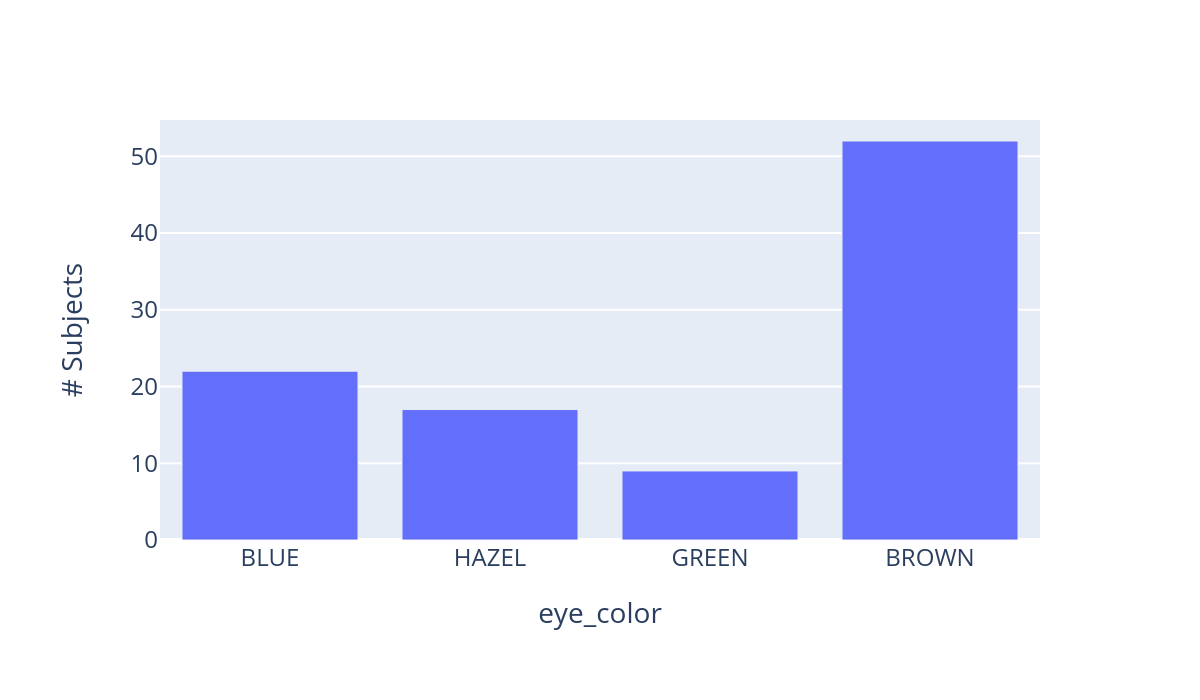
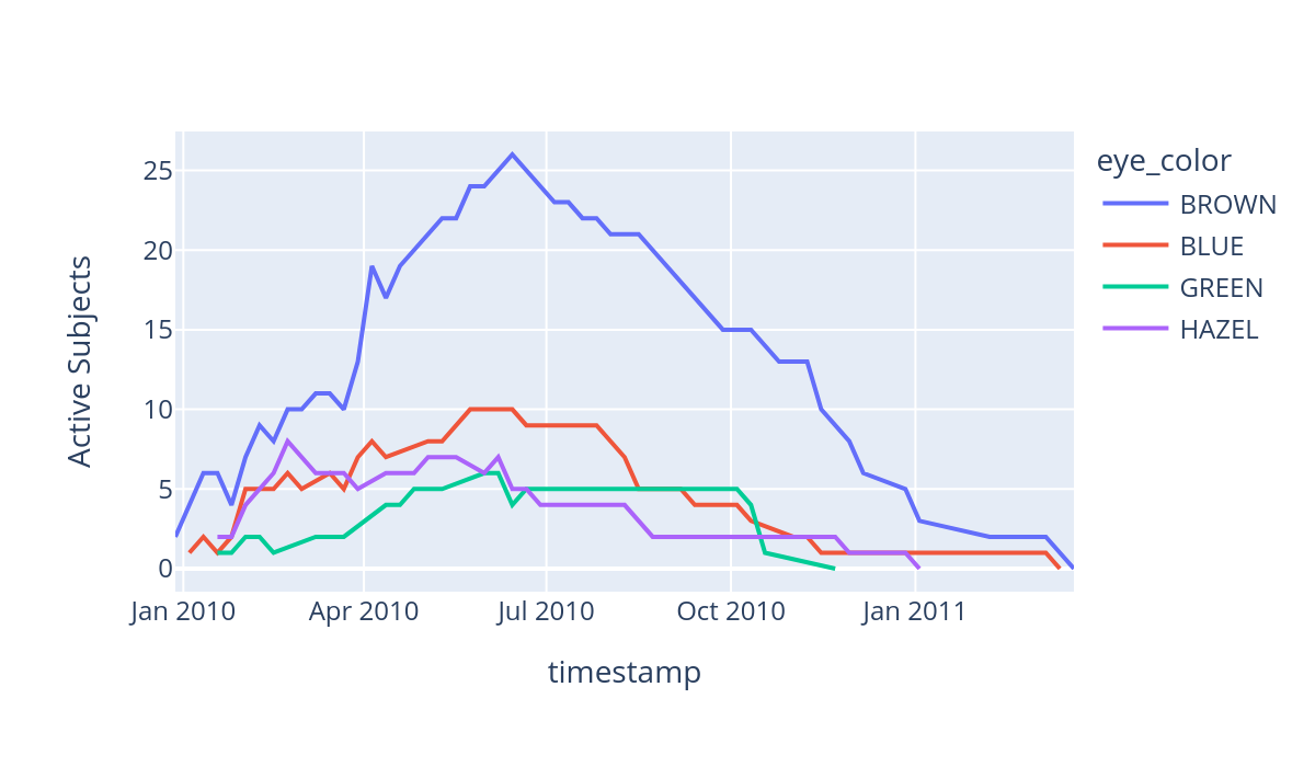
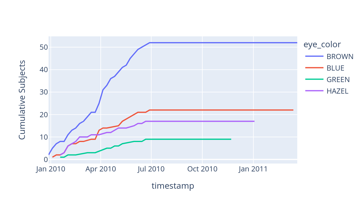
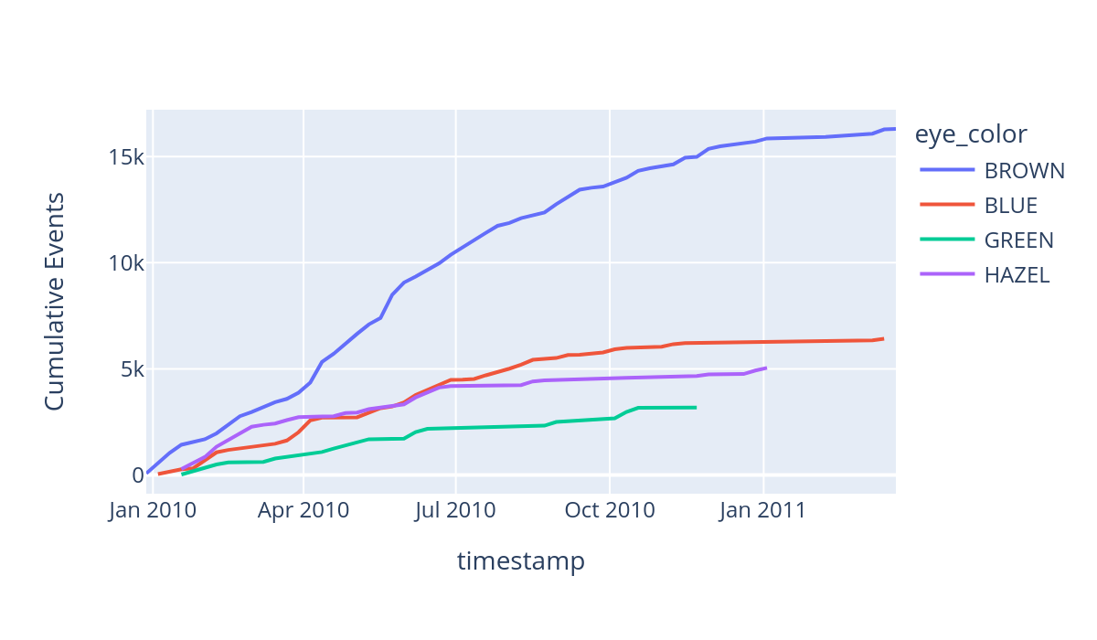
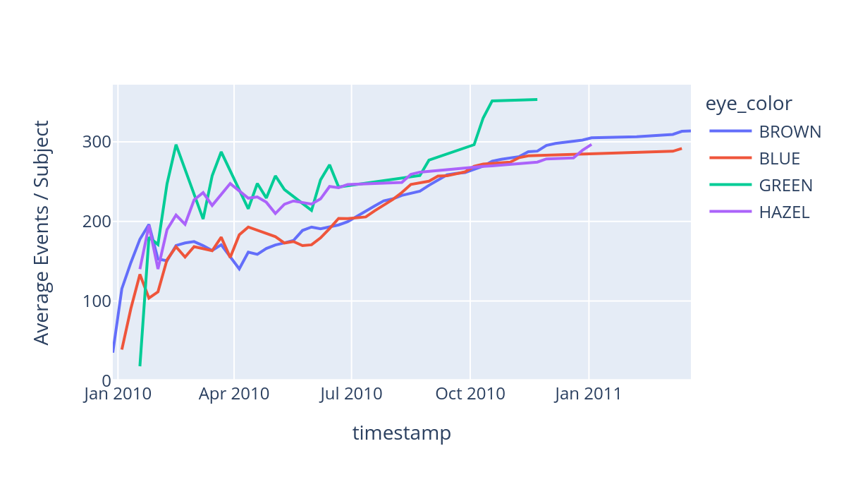
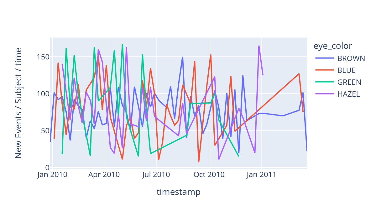
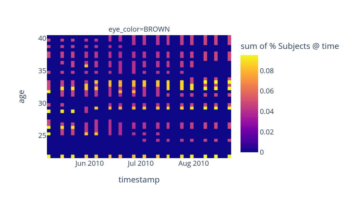
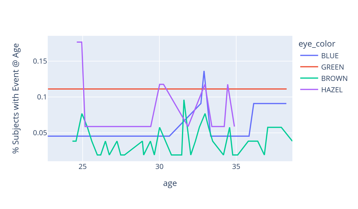
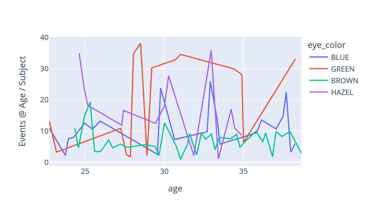
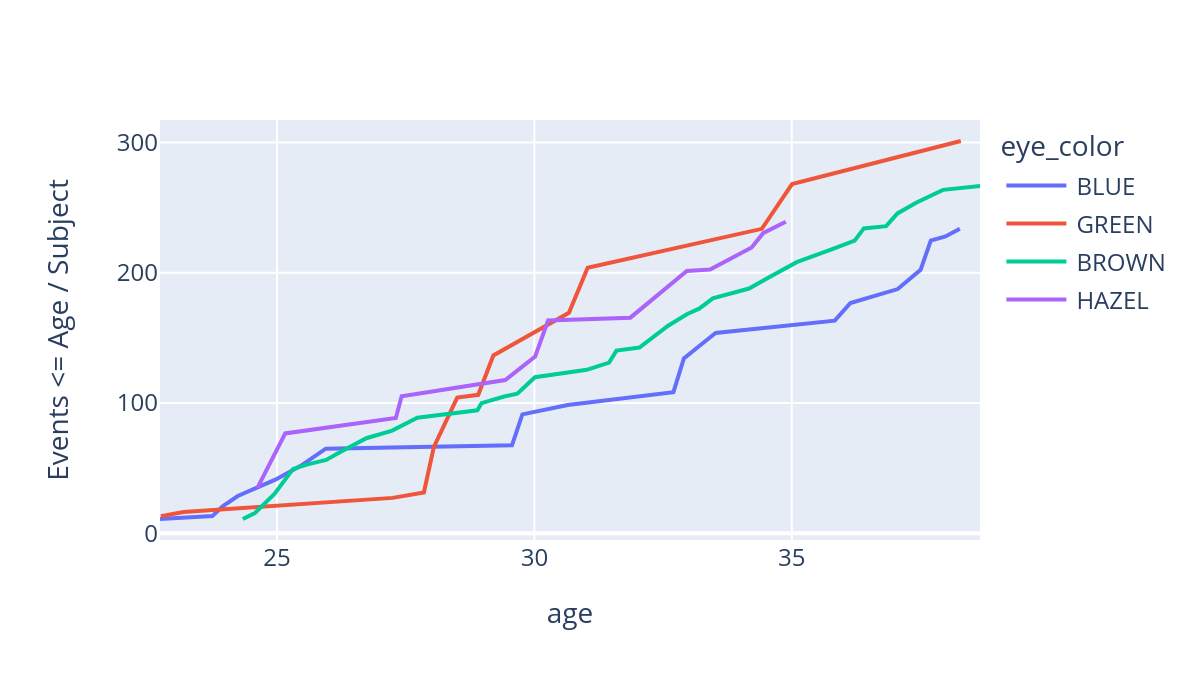
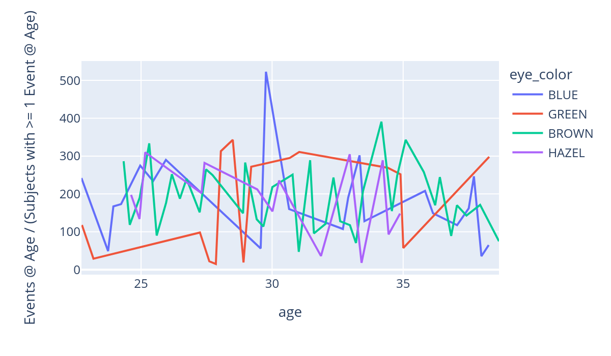
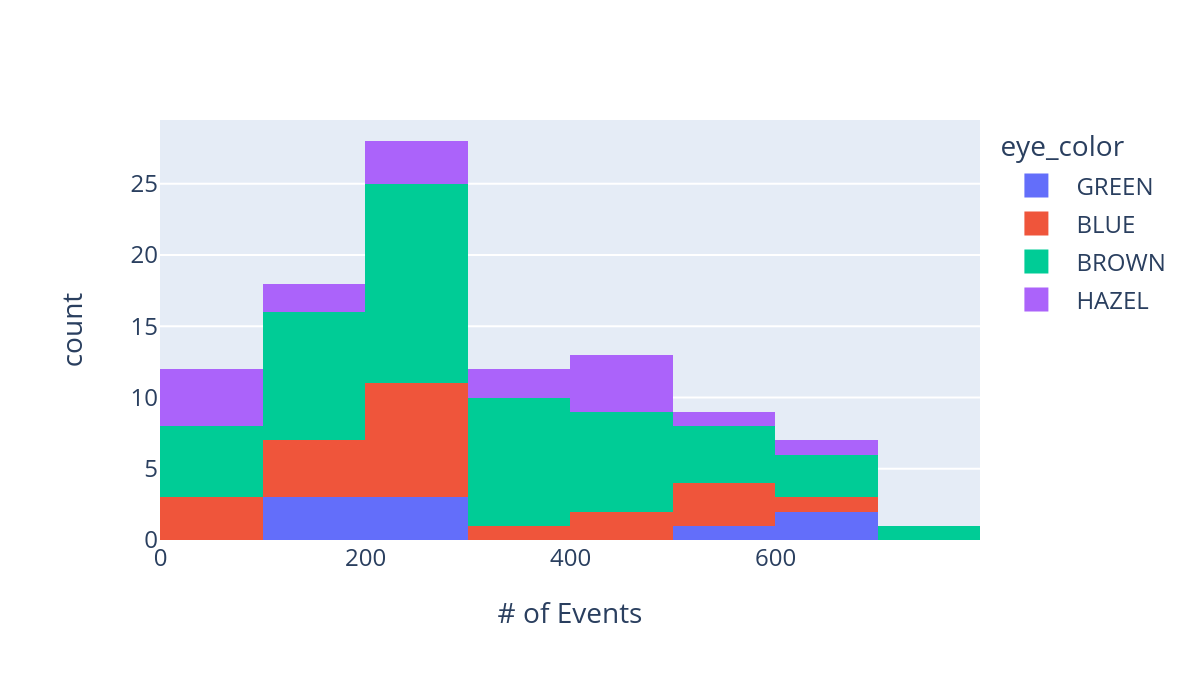
Automatic Task Cohort Extraction
Thanks to great work by Justin Xu, ESGPT will also soon support automatic, config-driven task cohort extraction and zero-shot labeler creation. See https://github.com/justin13601/ESGPTTaskQueryingPublic for more details!
Task configs: 
Training models
Next, we will show how you can train ESGPT style autoregressive models over these data. To begin, we need to know how these model architectures work:
How do model architectures work?
To see how model architectures work, consider the video tutorial below:
Training models with built in scripts
Now that you know how model architectures operate, let’s explore pre-training a toy model with the built-in pre-training script. It operates through a config file, much like the dataset building script does. Let’s see one such config file now:
[87]:
!cat sample_data/pretrain_CI.yaml
defaults:
  - pretrain_config
  - _self_

do_overwrite: false
seed: 1
config:
  do_use_learnable_sinusoidal_ATE: false
  do_split_embeddings: false
  static_embedding_mode: sum_all
  static_embedding_weight: 0.4
  dynamic_embedding_weight: 0.5
  do_normalize_by_measurement_index: false
  structured_event_processing_mode: conditionally_independent
  num_hidden_layers: 4
  seq_attention_types: ["global", "local"]
  seq_window_size: 4
  TTE_generation_layer_type: log_normal_mixture
  TTE_lognormal_generation_num_components: 2
  head_dim: 8
  num_attention_heads: 2
  attention_dropout: 0.2
  input_dropout: 0.2
  resid_dropout: 0.2
  intermediate_size: 128
optimization_config:
  init_lr: 0.0001
  end_lr_frac_of_init_lr: 0.01
  end_lr: null
  max_epochs: 2
  batch_size: 32
  validation_batch_size: 32
  lr_frac_warmup_steps: 0.05
  lr_decay_power: 2
  weight_decay: 0.2
  patience: null
  gradient_accumulation: null
  num_dataloader_workers: 1
data_config:
  save_dir: ???
  max_seq_len: 128
  min_seq_len: 4
pretraining_metrics_config:
  do_skip_all_metrics: false
  do_validate_args: true
  include_metrics:
    TRAIN:
      LOSS_PARTS: true
final_validation_metrics_config:
  n_auc_thresholds: 25
  do_skip_all_metrics: false
  do_validate_args: true
  include_metrics:
    TUNING:
      LOSS_PARTS: true
      TTE:
        MSE: true
        MSLE: true
      CLASSIFICATION:
        AUROC:
        - WEIGHTED
        ACCURACY: true
        AUPRC:
        - WEIGHTED
      REGRESSION:
        MSE: true
    HELD_OUT:
      LOSS_PARTS: true
      TTE:
        MSE: true
        MSLE: true
      CLASSIFICATION:
        AUROC:
        - WEIGHTED
        ACCURACY: true
      REGRESSION:
        MSE: true
        EXPLAINED_VARIANCE: true
        MSLE: true
trainer_config:
  accelerator: cpu
  devices: auto
  detect_anomaly: true
  log_every_n_steps: 1
experiment_dir: ???
wandb_logger_kwargs:
  name: null
  project: null
  team: null
  log_model: false
  do_log_graph: false
do_final_validation_on_metrics: true
do_use_filesystem_sharing: false
There are a variety of aspects to this config, including model parameters in the config section, optimization parameters in the optimization_config section, metrics specifications in the pretraining_ and final_validation_ metrics_config sections, PyTorch Lightning trainer parameters in the trainer_config, and weights and biases logger parameters in the wandb_logger_kwargs section.
To understand each of these different config section, inspect the documentation for the generative modeling pre-training main function and the overall model configuration classes.
To run a pre-training model, we’ll use the below script:
PYTHONPATH=$(pwd):$PYTHONPATH ./scripts/pretrain.py \
    --config-path="$(pwd)/sample_data/" \
    --config-name=pretrain_CI \
    "hydra.searchpath=[$(pwd)/configs]" \
    data_config.save_dir=$(pwd)/sample_data/processed/sample \
    experiment_dir=$(pwd)/sample_data/processed/PT_CI
[89]:
command = """\
PYTHONPATH=$(pwd):$PYTHONPATH ./scripts/pretrain.py \
    --config-path="$(pwd)/sample_data/" \
    --config-name=pretrain_CI \
    "hydra.searchpath=[$(pwd)/configs]" \
    data_config.save_dir=$(pwd)/sample_data/processed/sample \
    experiment_dir=$(pwd)/sample_data/processed/PT_CI
"""

command_out = subprocess.run(command, shell=True, capture_output=True)
print(command_out.stdout.decode())

if command_out.returncode == 1:
    print("Command Errored!")

print(command_out.stderr.decode())
WARNING: For a conditionally_independent model, measurements_per_dep_graph_level is not used; got []. Setting to None.
WARNING: For a conditionally_independent model, do_full_block_in_seq_attention is not used; got False. Setting to None.
WARNING: For a conditionally_independent model, do_full_block_in_dep_graph_attention is not used; got True. Setting to None.
WARNING: For a conditionally_independent model, dep_graph_window_size is not used; got 2. Setting to None.
Saving config files...
Writing to /home/mmd/Projects/EventStreamGPT/sample_data/processed/PT_CI/pretrain/2023-12-13_21-26-22/config.json
WARNING: For a conditionally_independent model, do_full_block_in_seq_attention is not used; got False. Setting to None.
WARNING: For a conditionally_independent model, do_full_block_in_dep_graph_attention is not used; got True. Setting to None.
WARNING: For a conditionally_independent model, dep_graph_window_size is not used; got 2. Setting to None.
Epoch 0: 100%|██████████| 3/3 [00:01<00:00,  2.51it/s, v_num=0]
Validation: |          | 0/? [00:00<?, ?it/s]
Validation:   0%|          | 0/1 [00:00<?, ?it/s]
Validation DataLoader 0:   0%|          | 0/1 [00:00<?, ?it/s]
Validation DataLoader 0: 100%|██████████| 1/1 [00:00<00:00, 24.12it/s]
Epoch 1: 100%|██████████| 3/3 [00:01<00:00,  2.90it/s, v_num=0]
Validation: |          | 0/? [00:00<?, ?it/s]
Validation:   0%|          | 0/1 [00:00<?, ?it/s]
Validation DataLoader 0:   0%|          | 0/1 [00:00<?, ?it/s]
Validation DataLoader 0: 100%|██████████| 1/1 [00:00<00:00, 27.66it/s]
Epoch 1: 100%|██████████| 3/3 [00:01<00:00,  2.42it/s, v_num=0]
WARNING: For a conditionally_independent model, do_full_block_in_seq_attention is not used; got False. Setting to None.
WARNING: For a conditionally_independent model, do_full_block_in_dep_graph_attention is not used; got True. Setting to None.
WARNING: For a conditionally_independent model, dep_graph_window_size is not used; got 2. Setting to None.
Validation DataLoader 0: 100%|██████████| 1/1 [00:00<00:00,  9.29it/s]
────────────────────────────────────────────────────────────────────────────────────────────────────────────────────────
          Validate metric                     DataLoader 0
────────────────────────────────────────────────────────────────────────────────────────────────────────────────────────
           tuning_HR_MSE                   1.9737292528152466
         tuning_HR_reg_NLL                  2.395521402359009
          tuning_TTE_MSE                       184308176.0
          tuning_TTE_MSLE                  0.5667116641998291
        tuning_TTE_reg_NLL                  4.943408012390137
     tuning_department_cls_NLL             0.6819429397583008
 tuning_department_macro_accuracy          0.6328583359718323
 tuning_department_micro_accuracy          0.6328583359718323
 tuning_department_weighted_AUROC          0.44778886437416077
tuning_department_weighted_accuracy        0.6736169457435608
     tuning_event_type_cls_NLL              2.867771625518799
 tuning_event_type_macro_accuracy          0.1593567281961441
 tuning_event_type_micro_accuracy           0.213429257273674
 tuning_event_type_weighted_AUROC          0.48839184641838074
tuning_event_type_weighted_accuracy        0.2134292721748352
        tuning_lab_name_MSE                0.19377931952476501
      tuning_lab_name_cls_NLL               0.693048357963562
  tuning_lab_name_macro_accuracy           0.5306316614151001
  tuning_lab_name_micro_accuracy           0.5306316018104553
      tuning_lab_name_reg_NLL              1.4089295864105225
  tuning_lab_name_weighted_AUROC           0.5106517672538757
 tuning_lab_name_weighted_accuracy         0.3423125743865967
            tuning_loss                    15.414828300476074
          tuning_temp_MSE                   2.123253107070923
        tuning_temp_reg_NLL                 2.424205780029297
────────────────────────────────────────────────────────────────────────────────────────────────────────────────────────
Testing DataLoader 0: 100%|██████████| 1/1 [00:00<00:00,  7.69it/s]
────────────────────────────────────────────────────────────────────────────────────────────────────────────────────────
             Test metric                         DataLoader 0
────────────────────────────────────────────────────────────────────────────────────────────────────────────────────────
           held_out_HR_MSE                     2.02217435836792
         held_out_HR_reg_NLL                   2.404747247695923
          held_out_TTE_MSE                        51963732.0
          held_out_TTE_MSLE                   0.37488314509391785
        held_out_TTE_reg_NLL                   4.53141975402832
     held_out_department_cls_NLL              0.6820839047431946
 held_out_department_macro_accuracy           0.6303570866584778
 held_out_department_micro_accuracy           0.6303571462631226
 held_out_department_weighted_AUROC           0.5057047605514526
held_out_department_weighted_accuracy         0.7216553688049316
     held_out_event_type_cls_NLL              2.8689451217651367
 held_out_event_type_macro_accuracy           0.04233268275856972
 held_out_event_type_micro_accuracy           0.2293144166469574
 held_out_event_type_weighted_AUROC           0.5220646858215332
held_out_event_type_weighted_accuracy         0.2293144166469574
        held_out_lab_name_MSE                 0.19800817966461182
      held_out_lab_name_cls_NLL               0.6928579211235046
  held_out_lab_name_macro_accuracy            0.5303657650947571
  held_out_lab_name_micro_accuracy            0.5303657650947571
      held_out_lab_name_reg_NLL               1.4523539543151855
  held_out_lab_name_weighted_AUROC            0.46757203340530396
 held_out_lab_name_weighted_accuracy          0.3350147306919098
            held_out_loss                     15.089038848876953
          held_out_temp_MSE                   2.1185483932495117
        held_out_temp_reg_NLL                 2.4566304683685303
────────────────────────────────────────────────────────────────────────────────────────────────────────────────────────
Saving final metrics...

Seed set to 1
You have turned on `Trainer(detect_anomaly=True)`. This will significantly slow down compute speed and is recommended only for model debugging.
GPU available: False, used: False
TPU available: False, using: 0 TPU cores
IPU available: False, using: 0 IPUs
HPU available: False, using: 0 HPUs
/home/mmd/mambaforge/envs/ESGPT_pl_0.18/lib/python3.10/site-packages/lightning/pytorch/trainer/connectors/logger_connector/logger_connector.py:67: Starting from v1.9.0, `tensorboardX` has been removed as a dependency of the `lightning.pytorch` package, due to potential conflicts with other packages in the ML ecosystem. For this reason, `logger=True` will use `CSVLogger` as the default logger, unless the `tensorboard` or `tensorboardX` packages are found. Please `pip install lightning[extra]` or one of them to enable TensorBoard support by default
Missing logger folder: /home/mmd/Projects/EventStreamGPT/sample_data/processed/PT_CI/pretrain/2023-12-13_21-26-22/model_checkpoints/lightning_logs

  | Name        | Type                               | Params
-------------------------------------------------------------------
0 | tte_metrics | ModuleDict                         | 0
1 | metrics     | ModuleDict                         | 0
2 | model       | CIPPTForGenerativeSequenceModeling | 24.0 K
-------------------------------------------------------------------
24.0 K    Trainable params
16        Non-trainable params
24.0 K    Total params
0.096     Total estimated model params size (MB)
/home/mmd/mambaforge/envs/ESGPT_pl_0.18/lib/python3.10/site-packages/lightning/pytorch/trainer/connectors/data_connector.py:441: The 'val_dataloader' does not have many workers which may be a bottleneck. Consider increasing the value of the `num_workers` argument` to `num_workers=7` in the `DataLoader` to improve performance.
/home/mmd/mambaforge/envs/ESGPT_pl_0.18/lib/python3.10/site-packages/lightning/pytorch/trainer/connectors/data_connector.py:441: The 'train_dataloader' does not have many workers which may be a bottleneck. Consider increasing the value of the `num_workers` argument` to `num_workers=7` in the `DataLoader` to improve performance.
`Trainer.fit` stopped: `max_epochs=2` reached.
Removed shared tensor {'encoder.input_layer.time_embedding_layer.cos_div_term'} while saving. This should be OK, but check by verifying that you don't receive any warning while reloading
/home/mmd/mambaforge/envs/ESGPT_pl_0.18/lib/python3.10/site-packages/lightning/pytorch/trainer/connectors/data_connector.py:441: The 'val_dataloader' does not have many workers which may be a bottleneck. Consider increasing the value of the `num_workers` argument` to `num_workers=7` in the `DataLoader` to improve performance.
/home/mmd/mambaforge/envs/ESGPT_pl_0.18/lib/python3.10/site-packages/lightning/pytorch/trainer/connectors/data_connector.py:441: The 'test_dataloader' does not have many workers which may be a bottleneck. Consider increasing the value of the `num_workers` argument` to `num_workers=7` in the `DataLoader` to improve performance.
We can see that the model ran successfully, though of course on this synthetic data it does not learn any final validation metrics that indicate better than chance performance. With this, however, you have seen how to structure your own pre-training configuration file to run pre-training models yourself! Check back soon for more details on this process and for examples of other modeling tasks ESGPT supports, such as fine-tuning, hyperparameter tuning, and generation or zero-shot inference!
[ ]: