MIMIC-IV Tutorial¶

Note that the raw code for this tutorial can also be found in this repository.

Tutorial Problem Set-up¶

In this user guide, we will follow the steps required to process data and produce foundation models over a small cohort from the MIMIC-IV dataset [JBS+23]

MIMIC-IV is a publicly available dataset consisting of the EHR data for all adult patients who were admitted to the emergency department (ED) or an intensive care unit (ICU) at Beth Israel Deaconess Medical Center (BIDMC) between 2008 and 2019. This dataset contains approximately 300,000 patients and consists of numerous modalities of health data, including diagnoses, laboratory test results, medications, in and out of hospital mortality, and many others, all localized continuously in time over all admissions of a single patient to the BIDMC.

Our task with these data is to build a generative model over the continuous-time, complex event stream data contained in MIMIC-IV. This can also be seen as a multi-variate marked temporal point process. In particular, given a sequence of complex events \(\vec x_1, \ldots, \vec x_N\) which occur at continuous times \(t_1, \ldots, t_N\), we wish to produce a model of the following probability distribution:

We will realize this through a transformer neural network architecture parametrized by \(\vec \theta\), such that \(f_{\vec \theta} (t_i, \vec x_i, \vec h_{i-1}) = p(t_i, \vec x_i | \vec h_{i-1})\). Note that here it may be the case that internal covariates of each event \(\vec x_i\) have internal causal dependencies. For example, if \(\vec x_i^{(j)}\) is used to denote the \(j\)th internal covariate of event \(i\), then \(p(\vec x_i | \vec h_{i-1}, t_i) \neq \prod_{j} p(\vec x_i^{(j)} | \vec h_{i-1}, t_i)\). Any full generative model will therefore need to account for these internal causal dependencies.

High-level Data Model¶

Before we detail the usage of this pipeline, we need to cover the general data model of the pipeline on the whole, which is illustrated in Figure 1. This data model can be broken down into three sections:

1. The core assumptions and internal data layout of the EFGPT pipeline

2. The pre-processing conventions and steps.

3. The final, deep-learning focused representation format and associated PyTorch Dataset data model.

We’ll walk through each of those in detail here.

Assumptions & Internal Data Layout¶

The EFGPT pipeline data model is composed of three entities, each of which are tracked internally in a separate dataframe.

Subjects¶

Subjects (e.g., patients) are data owners. Information at the per-subject level is non-time-varying. In Figure 1 (a), the sample patient record shown corresponds to a single subject \(S_1\); that subject has just one row in the subjects_df in Figure 1 (b).

Events¶

An event is an instance of something happening to a subject at a specific timestamp. Events are unique at the subject-timestamp level (i.e., no two events happen at the exact same time for the same subject). With the exception of a sentinel, categorical, “event type” variable, events do not have specially encoded information at the per-event level. Instead, events link in a one-to-many format to dynamic measurements. The first three visits of the subject in Figure 1 (a) each correspond to a single event (as all components of those visits are reported at the same timestamp in this example). As such, they each occupy a single row in the events_df dataframe in Figure 1 (b).

Dynamic Measurements¶

In EFGPT, Measurements, in general, refers to any observation or recorded metric about a subject. They can be static, in which case they are recorded at the per-subject level, not time-varying, and stored in the subjects dataframe, or they can be dynamic in which case they can occur arbitrarily in time and are recorded in a separate dataframe. Any observation that is recorded at a subject’s event is recorded as a row in the dynamic measurements dataframe, linked to events through an event ID. This allows us to maintain a sparse data structure and a minimal memory footprint overall, sa then other per-event details (e.g., event type, subject ID, and timestamp) do not need to be repeated if a single event has many associated dynamic measurements. In Fiure 1 (a), The various diagnostic codes, laboratory tests, procedures, etc. recorded in each of the first three visits will all be recorded as separate measurements, and occupy unique rows in dynamic_measurements_df in Figure 1 (b).

Pre-processing¶

During pre-processing, the EFGPT pipeline, in general, performances the following steps:

1. Converts input data types into minimal memory equivalents (e.g., strings to categorical data types, 64-bit signed integers for ID-spaces into *-bit unsigned integer types, etc.).

2. Applies pre-set censoring, outlier removal, and filtering over infrequently observed measurements to limit the input space.

3. Fits measurement vocabularies, outlier detection parameters, and normalization parameters over the categorical and numerical values observed in the train set.

4. Universally filters out infrequently observed categorical variables and outliers, normalizes numerical variables, and converts categorical variables to indices.

5. Produces deep-learning friendly representations for downstream use via the PytorchDataset class.

In this way, we can view the input of the entire EFGPT pipeline as the raw, pre-extraction input dataset, and the output as a pre-cached PyTorch Dataset ready-made for deep-learning use.

Dropped Data¶

Data can be dropped during the pre-processing pipeline in several ways:

1. Subjects who do not have sufficiently many events (unique timepoints) in the record can be dropped, depending on configuration parameters.

2. Measurements (e.g., entire columns) that are measured insufficiently frequently (again, pending configuration parameters) will be dropped.

3. Data elements (e.g., individual lab tests) that are observed insufficiently frequently will be re-mapped and aggregated to UNK vocabulary elements. No numerical measurements are dropped during such re-mappings, just re-assigned to the UNK key rather than the original key.

Deep-learning Representations¶

The deep learning representation is a polars dataframe written to disk. This dataframe has one row per subject, a set of sentinel columns that contain all observed information about each subject in a highly sparse format. In particular, this dataframe contains the following columns:

• subject_id: This column will be an unsigned integer type, and will have the ID of the subject for each row.

• start_time: This column will be a datetime type, and will contain the start time of the subject’s record.

• static_indices: This column is a ragged, sparse representation of the categorical static measurements observed for this subject. Each element of this column will itself be a list of unsigned integers corresponding to indices into the unified vocabulary for the static measurements observed for that subject.

• static_measurement_indices: This column corresponds in shape to static_indices, but contains unsigned integer indices into the unified measurement vocabulary, defining to which measurement each observation corresponds. It is of the same shape and of a consistent order as static_indices.

• time: This column is a ragged array of the time in minutes from the start time at which each event takes place. For a given row, the length of the array within this column corresponds to the number of events that subject has.

• dynamic_indices: This column is a doubly ragged array containing the indices of the observed values within the unified vocabulary per event per subject. Each subject’s data for this column consists of an array of arrays, each containing only the indices observed at each event.

• dynamic_measurement_indices This column is a doubly ragged array containing the indices of the observed measurements per event per subject. Each subject’s data for this column consists of an array of arrays, each containing only the indices of measurements observed at each event. It is of the same shape and of a consistent order as dynamic_indices.

• dynamic_values This column is a doubly ragged array containing the indices of the observed measurements per event per subject. Each subject’s data for this column consists of an array of arrays, each containing only the indices of measurements observed at each event. It is of the same shape and of a consistent order as dynamic_indices.

Data Extraction & Pre-processing¶

Now that we know the overarching data model for the pipeline, let us explore how we can actually build a dataset within it. The first entry point for our software is the data extraction and pre-processing component. To detail this pipeline, we will walk through the user’s process of creating a dataset and detail the technical inner workings of the pipeline at each stage.

Configuring the pipeline¶

The primary entry point for dataset building is through the scripts/build_dataset.py script. This script uses hydra to manage configuration and arguments, with the default configuration file for the script being found in configs/dataset_base.yml

Users can extend and specialize this configuration by defining their own yml file. To explain what the various configuration options are used for, we will rely on an example configuration file that is suitable for our working example over MIMIC-IV, shown below:

defaults:
  - dataset_base
  - _self_

subject_id_col: "subject_id"

connection_uri: "postgres://${oc.env:USER}:@localhost:5432/mimiciv"
min_los: 3
min_admissions: 1
inputs:
  patients:
    query: |-
      SELECT subject_id, gender, to_date((anchor_year-anchor_age)::CHAR(4), 'YYYY') AS year_of_birth
      FROM mimiciv_hosp.patients
      WHERE subject_id IN (
        SELECT long_icu.subject_id FROM (
          (
            SELECT subject_id FROM mimiciv_icu.icustays WHERE los > ${min_los}
          ) AS long_icu INNER JOIN (
            SELECT subject_id
            FROM mimiciv_hosp.admissions
            GROUP BY subject_id
            HAVING COUNT(*) > ${min_admissions}
          ) AS many_admissions
          ON long_icu.subject_id = many_admissions.subject_id
        )
      )
    must_have: ["gender", "year_of_birth"]
  admissions:
    query: "SELECT * FROM mimiciv_hosp.admissions"
    start_ts_col: "admittime"
    end_ts_col: ["dischtime", "deathtime"]
    start_columns:
      - "admission_type"
      - "admission_location"
      - "language"
      - "race"
      - "marital_status"
      - "insurance"
    end_columns: ["discharge_location"]
    event_type: ["VISIT", "ADMISSION", "DISCHARGE"]
  icu_stays:
    query: "SELECT * FROM mimiciv_icu.icustays"
    start_ts_col: "intime"
    end_ts_col: "outtime"
    start_columns: { "first_careunit": "careunit" }
    end_columns: { "last_careunit": "careunit" }
  diagnoses:
    query: |-
      SELECT
        admissions.subject_id,
        admissions.dischtime,
        ('ICD_' || diagnoses.icd_version || ' ' || TRIM(diagnoses.icd_code)) AS icd_code
      FROM (
        mimiciv_hosp.diagnoses_icd AS diagnoses JOIN mimiciv_hosp.admissions AS admissions
        ON admissions.hadm_id = diagnoses.hadm_id
      )
    ts_col: "dischtime"
  labs:
    query:
      - |-
        SELECT subject_id, charttime, (itemid || ' (' || valueuom || ')') AS lab_itemid, valuenum FROM
        mimiciv_hosp.labevents
      - |-
        SELECT subject_id, charttime, (itemid || ' (' || valueuom || ')') AS lab_itemid, valuenum FROM
        mimiciv_icu.chartevents
    ts_col: "charttime"
  infusions:
    query: |-
      SELECT
        icustays.subject_id,
        inputevents.itemid AS infusion_itemid,
        inputevents.totalamount,
        inputevents.patientweight,
        inputevents.starttime,
        inputevents.endtime
      FROM (
        mimiciv_icu.icustays AS icustays INNER JOIN mimiciv_icu.inputevents AS inputevents
        ON inputevents.stay_id = icustays.stay_id
      )
    start_ts_col: "starttime"
    end_ts_col: "endtime"
  procedures:
    query: |-
      SELECT
        icustays.subject_id,
        procedureevents.itemid AS procedure_itemid,
        procedureevents.starttime,
        procedureevents.endtime
      FROM (
        mimiciv_icu.icustays AS icustays INNER JOIN mimiciv_icu.procedureevents AS procedureevents
        ON procedureevents.stay_id = icustays.stay_id
      )
      WHERE procedureevents.ordercategorydescription IN ('Task', 'ContinuousProcess')
    start_ts_col: "starttime"
    end_ts_col: "endtime"
  medications:
    query: |-
      SELECT
        icustays.subject_id,
        emar.charttime,
        emar.medication
      FROM (
        mimiciv_icu.icustays AS icustays INNER JOIN mimiciv_hosp.emar AS emar
        ON emar.hadm_id = icustays.hadm_id
      )
      WHERE icustays.intime <= emar.charttime AND emar.charttime <= icustays.outtime
    ts_col: "charttime"

measurements:
  static:
    single_label_classification:
      patients: ["gender"]
  functional_time_dependent:
    age:
      functor: AgeFunctor
      necessary_static_measurements: { "year_of_birth": "timestamp" }
      kwargs:
        dob_col: "year_of_birth"
    time_of_day:
      functor: TimeOfDayFunctor
  dynamic:
    multi_label_classification:
      admissions:
        - "admission_type"
        - "admission_location"
        - "language"
        - "race"
        - "marital_status"
        - "insurance"
        - "discharge_location"
      icu_stays: ["careunit"]
      diagnoses: ["icd_code"]
      procedures: ["procedure_itemid"]
      medications: ["medication"]
    multivariate_regression:
      labs: [["lab_itemid", "valuenum"]]
      infusions: [["infusion_itemid", "totalamount"]]
    univariate_regression:
      infusions: ["patientweight"]

save_dir: "${oc.env:PROJECT_DATA_DIR}/${cohort_name}"
outlier_detector_config:
  stddev_cutoff: 4.0
min_valid_vocab_element_observations: 25
min_valid_column_observations: 50
min_true_float_frequency: 0.1
min_unique_numerical_observations: 25
min_events_per_subject: 20
agg_by_time_scale: "2h"

With this configuration file saved to path .../configs/dataset.yml, and with EFGPT_PATH defined to point to the root of the EFGPT repo, then the dataset pipeline can be built with the command

PYTHONPATH="$EFGPT_PATH:$PYTHONPATH" python \
	$EFGPT_PATH/scripts/build_dataset.py \
	--config-path=$(pwd)/configs \
	--config-name=dataset \
	"hydra.searchpath=[$EFGPT_PATH/configs]" [configuration args...]

The only mandatory command line configuration argument with this setup is the cohort_name argument. As can be seen in the default dataset_base.yml configuration file in the base library, it’s value is set to the sentinel OmegaConf “MISSING” value, ???, so must be overwritten either in the config file or on the command line.

Working through this example, we can see there are several four key sections to this configuration file / command:

Hydra-specific parameters¶

The defaults: block at the top is a Hydra specific inclusion, and ensures the script knows to merge this configuration file. Similarly, the hydra.searchpath=[$EFGPT_PATH/confgis] command line argument also ensures Hydra knows to look for the base config in the EFGPT repository’s configs path.

Inputs¶

This section of the config defines the input data sources from which raw data should be extracted. It consists of two parts: a set of global parameters that are used across all input sources and a collection of specific individual input sources, with configuration information detailing how to extract them.

Global Parameters¶

The global parameters, in this example, consist of the following:

subject_id_col: subject_id
connection_uri: postgres://${oc.env:USER}:@localhost:5432/mimiciv

min_los: 3
min_admissions: 1

Of these, the subject_id_col is the only mandatory parameter, as it details what (single) ID column is used to identify subjects uniquely across all input sources (i.e., all input sources must have a column with this name that holds the unique ID of the subject). The connection_uri parameter is not mandatory, but it is a software recognized keyword parameter that is used to provide the default connection URI for all database queries in the config (if per-query URIs are not provided).

The remaining two parameters are custom parameters that are only used in the MIMIC-IV example, to make it easier to configure on the fly. This is not a weakness of the configuration language; in fact, it is a strength. Any dataset can have dataset-specific configuration parameters in addition to the default one if they make it easier to specify the dataset you want (in the bounds of the configuration file). For example, through Hydra’s interpolation syntax, we are able to use these parameters to control the cohort selection query in the patients input block:

patients:
  query: |-
    ... # Omitted for brevity
    WHERE subject_id IN (
      SELECT long_icu.subject_id FROM (
        (
          SELECT subject_id FROM mimiciv_icu.icustays WHERE los > ${min_los}
        ) AS long_icu INNER JOIN (
          SELECT subject_id
          FROM mimiciv_hosp.admissions
          GROUP BY subject_id
          HAVING COUNT(*) > ${min_admissions}
        ) AS many_admissions
    ... # Omitted for brevity

This allows us to overwrite those parameters in a given run on the command line, with, for example, ... min_los=1 min_admissions=2.

Note that these parameters drive the actual exclusion/inclusion criteria of subjects in our dataset. In particular, these queries drop all subjects who don’t have sufficient admissions or admissions with sufficiently long ICU stays from the dataset, thereby filtering the full MIMIC-IV dataset down from the 300k patients present in the full data to only the 12k patients who remain in our final cohort. Relatedly, the query for laboratory test values, shown below, conjoins laboratory test names and their units of measure, which can result in some laboratory test values being remapped to UNKs if they do not occur sufficiently frequently with select units.

labs:
  query:
    - |-
      SELECT subject_id, charttime, (itemid || ' (' || valueuom || ')') AS lab_itemid, valuenum FROM
      mimiciv_hosp.labevents
    - |-
      SELECT subject_id, charttime, (itemid || ' (' || valueuom || ')') AS lab_itemid, valuenum FROM
      mimiciv_icu.chartevents
  ts_col: charttime

Per-input Blocks:¶

The input-database specific input blocks define the raw datasets that we should read to build the output dataset. They take the form of the nested keys and values within the inputs key. Each key defines a named input data-table from which raw data will be extracted, and the value is a specific configuration object to partially define that extraction process. Below is the full documentation of each parameter allowed in these input blocks:

Measurements¶

The measurements block defines not from what input sources we should read, but what output measurements we should include in our dataset. It has a very simple structure, consisting of a nested dictionary. The outermost layer of this structure has a key for each valid temporal mode a measurement can take: static, dynamic, or functional_time_dependent.

Within the static and dynamic keys, there is yet another nested dictionary, where the outer keys correspond to the permitted measurement modalities: single_label_classification, multi_label_classification, univariate_regression, and multivariate_regression. Within each of these, there is one final dictionary, whose keys are the names of input sources from which measurements should be pulled and whose values are the list of measurement names that should be extracted from said input source. Note that these names are the output names of the measurements, which are not necessarily the same as the raw column names in the input dataset.

The functional_time_dependent key has a similar, but slightly different structure. Rather than having a nested dictionary of measurements by input sources by modalities, it has an inner dictionary which has the desired output functional_time_dependent measurement names as keys and whose values store the configuration options for those measurement’s configuration files.

Core configuration parameters¶

The core configuration block, reporduced below, contains any speciality DatasetConfig parameters.

save_dir: ${oc.env:PROJECT_DATA_DIR}/${cohort_name}
outlier_detector_config:
  stddev_cutoff: 4.0
min_valid_vocab_element_observations: 25
min_valid_column_observations: 50
min_true_float_frequency: 0.1
min_unique_numerical_observations: 25
min_events_per_subject: 20
agg_by_time_scale: 2h

These parameters showcase several aspects of the configuration language. Firstly, the save_dir specification showcases Hydra/OmegaConfg’s Interpolation Capabilities.

Secondly, we can see in addition several other aspects of the configuration being specialized; this configuration specifies that variables more than 4 standard deviations away from the mean should be considered outliers, that columns/measurements must be observed 50 times to be included at all, that there must be at least 10% of values actually being floating point for a numerical measure to not be re-cast as integer-valued, for a numerical column to need at least 25 unique values to not be re-cast as categorical, to only retain subjects who have at least 20 subjects, and to aggregate all events together into 2-hour buckets.

Outside of the core measurements and input blocks, any remaining parameters that are elements of the DatasetConfig object will be incorporated into the final config and reflected in pre-processing, etc.

Using the Dataset¶

Now that the dataset is pre-built, we can use it. The dataset can be used directly (not through the PyTorch Dataset format) for several applications. Here, we highlight two:

1. Dataset exploration & visualization.

2. Building task dataframes for fine-tuning. In this step, we’ll also show how to craft zero-shot labelers, though this doesn’t really rely on the dataset class.

Dataset Exploration & Visualization¶

Event Stream GPT comes with some pre-built utilities to aid in exploring and understanding datasets, through the visualize and describe methods. Calling these methods on a freshly re-loaded MIMIC-IV cohort yields the following:

Loading subjects from /n/data1/hms/dbmi/zaklab/RAMMS/data/MIMIC_IV/ESD_06-13-23_150GB_10cpu-1/subjects_df.parquet...
Loading events from /n/data1/hms/dbmi/zaklab/RAMMS/data/MIMIC_IV/ESD_06-13-23_150GB_10cpu-1/events_df.parquet...
Loading dynamic_measurements from /n/data1/hms/dbmi/zaklab/RAMMS/data/MIMIC_IV/ESD_06-13-23_150GB_10cpu-1/dynamic_measurements_df.parquet...
Dataset has 12.1 thousand subjects, with 2.8 million events and 222.4 million measurements.
Dataset has 17 measurements:
gender: static, single_label_classification observed 100.0%
Vocabulary:
  3 elements, 0.0% UNKs
  Frequencies: █▁
  Elements:
    (55.2%) M
    (44.8%) F

admission_type: dynamic, multi_label_classification [...]
Vocabulary:
  10 elements, 0.0% UNKs
  Frequencies: █▃▃▂▂▂▁▁▁
  Examples:
    (44.2%) EW EMER.
    (14.5%) OBSERVATION ADMIT
    (10.7%) EU OBSERVATION
    ...
    (2.8%) ELECTIVE
    (1.5%) AMBULATORY OBSERVATION

admission_location: dynamic, [...]
Vocabulary:
  12 elements, 0.0% UNKs
  Frequencies: █▄▂▁▁▁▁▁▁▁▁
  Examples:
    (53.4%) EMERGENCY ROOM
    (23.5%) PHYSICIAN REFERRAL
    (11.0%) TRANSFER FROM HOSPITAL
    ...
    (0.1%) INFORMATION NOT AVAILABLE
    (0.1%) AMBULATORY SURGERY TRANSFER

language: dynamic, multi_label_classification observed 2.5%
Vocabulary:
  3 elements, 0.0% UNKs
  Frequencies: █▁
  Elements:
    (89.1%) ENGLISH
    (10.9%) ?

race: dynamic, multi_label_classification observed 2.5%
Vocabulary:
  34 elements, 0.0% UNKs
  Frequencies: █▃▁▁▁▁▁▁▁▁▁▁▁▁▁▁▁▁▁▁▁▁▁▁▁▁▁▁▁▁▁▁▁
  Examples:
    (64.6%) WHITE
    (15.0%) BLACK/AFRICAN AMERICAN
    (2.7%) OTHER
    ...
    (0.1%) NATIVE HAWAIIAN OR OTHER PACIFIC ISLANDER
    (0.0%) HISPANIC/LATINO - HONDURAN

marital_status: dynamic, multi_label_classification [...]
Vocabulary:
  5 elements, 0.0% UNKs
  Frequencies: █▆▂▁
  Elements:
    (45.7%) MARRIED
    (33.6%) SINGLE
    (12.6%) WIDOWED
    (8.1%) DIVORCED

insurance: dynamic, multi_label_classification observed 2.5%
Vocabulary:
  4 elements, 0.0% UNKs
  Frequencies: █▇▁
  Elements:
    (49.4%) Medicare
    (42.0%) Other
    (8.5%) Medicaid

discharge_location: dynamic, [...]
Vocabulary:
  13 elements, 0.0% UNKs
  Frequencies: █▇▅▂▂▂▁▁▁▁▁▁
  Examples:
    (31.9%) HOME
    (29.1%) HOME HEALTH CARE
    (18.7%) SKILLED NURSING FACILITY
    ...
    (0.4%) OTHER FACILITY
    (0.1%) ASSISTED LIVING

careunit: dynamic, multi_label_classification observed 1.9%
Vocabulary:
  10 elements, 0.0% UNKs
  Frequencies: █▆▅▄▄▃▁▁▁
  Examples:
    (25.7%) Medical Intensive Care Unit (MICU)
    (17.6%) Medical/Surgical Intensive Care Unit (MICU/SICU)
    (15.5%) Surgical Intensive Care Unit (SICU)
    ...
    (1.9%) Neuro Surgical Intensive Care Unit (Neuro SICU)
    (1.4%) Neuro Stepdown

icd_code: dynamic, multi_label_classification observed 2.5%
Vocabulary:
  2993 elements, 6.0% UNKs
  Frequencies: █▂▂▁▁▁▁▁▁▁▁▁▁▁▁▁▁▁▁▁▁▁▁▁▁▁▁▁▁▁▁▁▁▁▁▁▁▁▁▁▁▁▁▁
  Examples:
    (1.5%) ICD_9 4019
    (1.2%) ICD_9 2724
    (1.1%) ICD_9 4280
    ...
    (0.0%) ICD_10 D594
    (0.0%) ICD_10 C775

procedure_itemid: dynamic, multi_label_classification [...]
Vocabulary:
  141 elements, 0.0% UNKs
  Frequencies: █▄▃▂▂▂▂▂▁▁▁▁▁▁▁▁▁▁▁▁▁▁▁▁▁▁▁▁▁▁▁▁▁▁▁
  Examples:
    (11.5%) 225459
    (10.6%) 224275
    (6.0%) 224277
    ...
    (0.0%) 226237
    (0.0%) 228228

medication: dynamic, multi_label_classification [...]
Vocabulary:
  795 elements, 0.3% UNKs
  Frequencies: █▂▁▁▁▁▁▁▁▁▁▁▁▁▁▁▁▁▁▁▁▁▁▁▁▁▁▁▁▁▁▁▁▁▁▁▁▁▁▁▁▁
  Examples:
    (9.0%) Sodium Chloride 0.9% Flush
    (7.7%) Insulin
    (4.5%) Heparin
    ...
    (0.0%) ChlordiazePOXIDE
    (0.0%) Basiliximab

lab_itemid: dynamic, multivariate_regression observed 94.8%
Value Types:
  396 integer
  279 float
  179 dropped
  94 categorical_integer
  39 categorical_float
Vocabulary:
  1152 elements, 0.0% UNKs
  Frequencies: █▂▂▁▁▁▁▁▁▁▁▁▁▁▁▁▁▁▁▁▁▁▁▁▁▁▁▁▁▁▁▁▁▁▁▁▁▁▁▁▁▁▁
  Examples:
    (5.3%) 220045 (bpm)
    (5.2%) 220210 (insp/min)
    (5.2%) 220277 (%)
    ...
    (0.0%) 228624 (cm)__EQ_3.0
    (0.0%) 227645 (min)__EQ_15

infusion_itemid: dynamic, multivariate_regression [...]
Value Types:
  137 categorical_integer
  81 integer
  64 dropped
  1 categorical_float
Vocabulary:
  527 elements, 0.1% UNKs
  Frequencies: █▂▁▁▁▁▁▁▁▁▁▁▁▁▁▁▁▁▁▁▁▁▁▁▁▁▁▁▁▁▁▁▁▁▁▁▁▁▁▁▁▁▁▁
  Examples:
    (15.9%) 225158
    (12.9%) 220949
    (6.9%) 225943
    ...
    (0.0%) 221289__EQ_247
    (0.0%) 221036__EQ_840

patientweight: dynamic, univariate_regression observed 47.0%
Value is a float

age: functional_time_dependent, univariate_regression [...]
Value is a float

time_of_day: functional_time_dependent, [...]
Vocabulary:
  5 elements, 0.0% UNKs
  Frequencies: █▆▅▁
  Elements:
    (36.9%) PM
    (28.1%) AM
    (24.9%) EARLY_AM
    (10.0%) LATE_PM

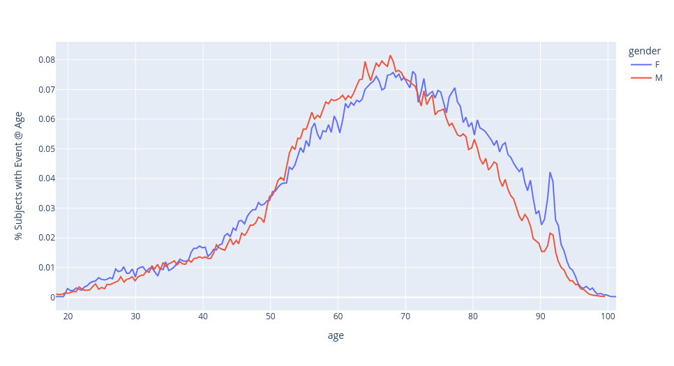% of subjects with an event by age and gender.

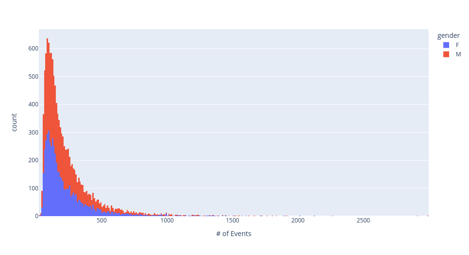Total number of events per subject, by gender.

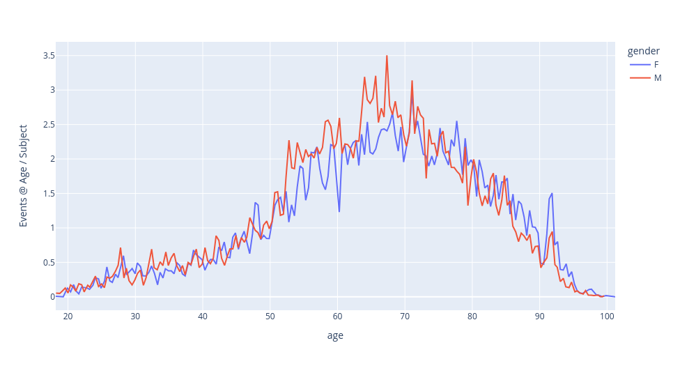Events per subject at age, by gender.

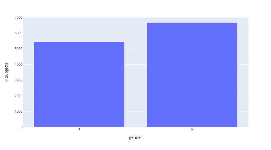Subject gender breakdown

Building Task DataFrames (& Labelers!)¶

In order to assess performance on downstream tasks over these data, we need to define “task dataframes” that describe these downstream targets. This takes two forms: first, a simple task dataframe which defines a task schema and cohort, and second, a zero-shot labeling function that can infer empirical task labels from generated batches. We describe both options here.

Task DataFrames¶

Task dataframes in our setting are built using Polars queries over the internal dataframes of the dataset object. These can be seen in the tutorial repository notebook, here.

The logic to construct these task dataframes is relatively simple, and we hope to soon add functionality to allow these to be configurable without needing to write explicit code. In this example, we define two tasks: 30-day readmission risk prediction and in-hospital mortality prediction. Both can be found in the notebook linked above, but we will show a sample here demonstrating the construction, and final schema, of the task dataframe for readmission risk prediction below.

# %%time
# %%memit

import os
from pathlib import Path

import polars as pl

from EventStream.data.dataset_polars import Dataset

COHORT_NAME = "MIMIC_IV/ESD_06-13-23_150GB_10cpu-1"
PROJECT_DIR = Path(os.environ["PROJECT_DIR"])
DATA_DIR = PROJECT_DIR / "data" / COHORT_NAME
assert DATA_DIR.is_dir()

TASK_DF_DIR = DATA_DIR / "task_dfs"
TASK_DF_DIR.mkdir(exist_ok=True, parents=False)

ESD = Dataset.load(DATA_DIR)


def has_event_type(type_str: str) -> pl.Expr:
    event_types = pl.col("event_type").cast(pl.Utf8).str.split("&")
    return event_types.list.contains(type_str)


events_df = ESD.events_df.lazy()

readmission_30d = (
    events_df.with_columns(
        has_event_type("DISCHARGE").alias("is_discharge"), has_event_type("ADMISSION").alias("is_admission")
    )
    .filter(pl.col("is_discharge") | pl.col("is_admission"))
    .sort(["subject_id", "timestamp"], descending=False)
    .with_columns(
        pl.when(pl.col("is_admission"))
        .then(pl.col("timestamp"))
        .otherwise(None)
        .alias("admission_time")
        .cast(pl.Datetime)
    )
    .with_columns(
        pl.col("admission_time")
        .fill_null(strategy="backward")
        .over("subject_id")
        .alias("next_admission_time"),
        pl.col("admission_time")
        .fill_null(strategy="forward")
        .over("subject_id")
        .alias("prev_admission_time"),
    )
    .with_columns(
        ((pl.col("next_admission_time") - pl.col("timestamp")) < pl.duration(days=30))
        .fill_null(False)
        .alias("30d_readmission")
    )
    .filter(pl.col("is_discharge"))
)

readmission_30d_all = readmission_30d.select(
    "subject_id",
    pl.lit(None).cast(pl.Datetime).alias("start_time"),
    pl.col("timestamp").alias("end_time"),
    "30d_readmission",
)

readmission_30d_all.collect().write_parquet(TASK_DF_DIR / "readmission_30d_all.parquet")

prevalence = readmission_30d_all.select(pl.col("30d_readmission").mean()).collect().item()
print(f"The {COHORT_NAME} cohort has a {prevalence*100:.1f}% 30d readmission prevalence.")

# Loading events from \
# /n/data1/hms/dbmi/zaklab/RAMMS/data/MIMIC_IV/ESD_06-13-23_150GB_10cpu-1/events_df.parquet...
# The MIMIC_IV/ESD_06-13-23_150GB_10cpu-1 cohort has a 32.6% 30d readmission prevalence.
# peak memory: 912.86 MiB, increment: 496.57 MiB
# CPU times: user 7.19 s, sys: 1.34 s, total: 8.53 s
# Wall time: 4.55 s

Zero-shot Labelers¶

Zero-shot labelers are user-defined functors that can compute an empirical label for a generated batch of data, to enable zero-shot evaluation of an Event Stream GPT. These are fully documented in the source code for this working example, but we also highlight one example labeler below, for in-hospital mortality prediction.

import torch

from EventStream.data.pytorch_dataset import PytorchBatch
from EventStream.transformer.model_output import get_event_types
from EventStream.transformer.zero_shot_labeler import Labeler


def masked_idx_in_set(
    indices_T: torch.LongTensor, indices_set: set[int], mask: torch.BoolTensor
) -> torch.BoolTensor:
    return torch.where(mask, torch.any(torch.stack([(indices_T == i) for i in indices_set], 0), dim=0), False)


class TaskLabeler(Labeler):
    def __call__(self, batch: PytorchBatch, input_seq_len: int) -> tuple[torch.LongTensor, torch.BoolTensor]:
        gen_mask = batch.event_mask[:, input_seq_len:]
        gen_measurements = batch.dynamic_measurement_indices[:, input_seq_len:, :]
        gen_indices = batch.dynamic_indices[:, input_seq_len:, :]

        gen_event_types = get_event_types(
            gen_measurements,
            gen_indices,
            self.config.measurements_idxmap["event_type"],
            self.config.vocab_offsets_by_measurement["event_type"],
        )

        # gen_event_types is of shape [batch_size, sequence_length]

        discharge_indices = {
            i for et, i in self.config.event_types_idxmap.items() if ("DISCHARGE" in et.split("&"))
        }
        death_indices = {i for et, i in self.config.event_types_idxmap.items() if ("DEATH" in et.split("&"))}

        is_discharge = masked_idx_in_set(gen_event_types, discharge_indices, gen_mask)
        is_death = masked_idx_in_set(gen_event_types, death_indices, gen_mask)

        no_discharge = (~is_discharge).all(dim=1)
        first_discharge = torch.argmax(is_discharge.float(), 1)
        first_discharge = torch.where(no_discharge, batch.sequence_length + 1, first_discharge)

        no_death = (~is_death).all(dim=1)
        first_death = torch.argmax(is_death.float(), 1)
        first_death = torch.where(no_death, batch.sequence_length + 1, first_death)

        pred_discharge = torch.where(
            (~no_discharge) & (first_discharge < first_death),
            torch.ones_like(first_discharge),
            torch.zeros_like(first_discharge),
        )
        pred_death = torch.where(
            (~no_death) & (first_death <= first_discharge),
            torch.ones_like(first_death),
            torch.zeros_like(first_discharge),
        )

        # MAKE SURE THIS ORDER MATCHES THE EXPECTED LABEL VOCAB
        # Accessible in self.config.label2id
        pred_labels = torch.stack([pred_discharge, pred_death], 1)
        unknown_pred = (pred_discharge == 0) & (pred_death == 0)

        return pred_labels, unknown_pred

After defining these labelers, one simply needs to copy them into the task dataframes folder for the corresponding dataset, and they can be used for evaluation with no issue.

Pre-training Models¶

Hyperparameter Tuning¶

Weights and Biases Sweep¶

The configuration file used in our working example can be found below. It specifies a total of 8 possible options for measurements_per_dep_graph_level, specific to the MIMIC dataset. Otherwise, it relies on default parameter selections from the config/hyperparameter_sweep_base.yaml file.

defaults:
  - hyperparameter_sweep_base
  - _self_

cohort_name: ???
project: ${oc.env:PROJECT_NAME}
program: ${oc.env:EVENT_STREAM_PATH}/scripts/pretrain.py

parameters:
  experiment_dir:
    value: ${oc.env:PROJECT_DIR}/models/hyperparameter_search/${cohort_name}/sweep_${now:%m-%d-%y_%H-%M-%S}
  num_dataloader_workers:
    value: 15
  data_config:
    save_dir:
      value: ${oc.env:PROJECT_DIR}/data/MIMIC_IV/${cohort_name}
  config:
    measurements_per_dep_graph_level:
      values:
        - - ["age", "time_of_day"]
          - ["event_type"]
          - [
              "patientweight",
              "admission_type",
              "admission_location",
              "race",
              "language",
              "marital_status",
              "insurance",
              "careunit",
              ["lab_itemid", "categorical_only"],
              ["infusion_itemid", "categorical_only"],
            ]
          - [
              ["lab_itemid", "numerical_only"],
              ["infusion_itemid", "numerical_only"],
            ]
          - ["procedure_itemid", "medication", "icd_code", "discharge_location"]
        - - ["age", "time_of_day"]
          - ["event_type"]
          - [
              "race",
              "language",
              "marital_status",
              "insurance",
              "admission_type",
            ]
          - ["admission_location", "careunit"]
          - [
              ["lab_itemid", "categorical_only"],
              ["infusion_itemid", "categorical_only"],
              "patientweight",
            ]
          - [
              ["lab_itemid", "numerical_only"],
              ["lab_itemid", "numerical_only"],
              "procedure_itemid",
              "medication",
              "icd_code",
              "discharge_location",
            ]
        - - ["age", "time_of_day"]
          - ["event_type"]
          - [
              "race",
              "language",
              "marital_status",
              "insurance",
              "admission_type",
            ]
          - ["admission_location", "careunit"]
          - [
              "lab_itemid",
              "infusion_itemid",
              "patientweight",
              "procedure_itemid",
              "medication",
              "icd_code",
              "discharge_location",
            ]
        - - ["age", "time_of_day"]
          - ["event_type"]
          - [
              "lab_itemid",
              "infusion_itemid",
              "patientweight",
              "procedure_itemid",
              "medication",
              "icd_code",
              "race",
              "language",
              "marital_status",
              "insurance",
              "admission_type",
              "admission_location",
              "careunit",
              "discharge_location",
            ]
        - - ["age", "time_of_day"]
          - [
              "event_type",
              "patientweight",
              "admission_type",
              "admission_location",
              "race",
              "language",
              "marital_status",
              "insurance",
              "careunit",
              ["lab_itemid", "categorical_only"],
              ["infusion_itemid", "categorical_only"],
            ]
          - [
              ["lab_itemid", "numerical_only"],
              ["infusion_itemid", "numerical_only"],
            ]
          - ["procedure_itemid", "medication", "icd_code", "discharge_location"]
        - - ["age", "time_of_day"]
          - [
              "event_type",
              "race",
              "language",
              "marital_status",
              "insurance",
              "admission_type",
            ]
          - ["admission_location", "careunit"]
          - [
              ["lab_itemid", "categorical_only"],
              ["infusion_itemid", "categorical_only"],
              "patientweight",
            ]
          - [
              ["lab_itemid", "numerical_only"],
              ["lab_itemid", "numerical_only"],
              "procedure_itemid",
              "medication",
              "icd_code",
              "discharge_location",
            ]
        - - ["age", "time_of_day"]
          - [
              "event_type",
              "race",
              "language",
              "marital_status",
              "insurance",
              "admission_type",
            ]
          - ["admission_location", "careunit"]
          - [
              "lab_itemid",
              "infusion_itemid",
              "patientweight",
              "procedure_itemid",
              "medication",
              "icd_code",
              "discharge_location",
            ]
        - - ["age", "time_of_day"]
          - [
              "event_type",
              "lab_itemid",
              "infusion_itemid",
              "patientweight",
              "procedure_itemid",
              "medication",
              "icd_code",
              "race",
              "language",
              "marital_status",
              "insurance",
              "admission_type",
              "admission_location",
              "careunit",
              "discharge_location",
            ]

Template Analysis Report¶

A template hyperparameter sweep analysis report can be found here. Users can clone this into their own weights and biases projects to further accelerate hyperparameter tuning analysis. Samples of its outputs can be found below.

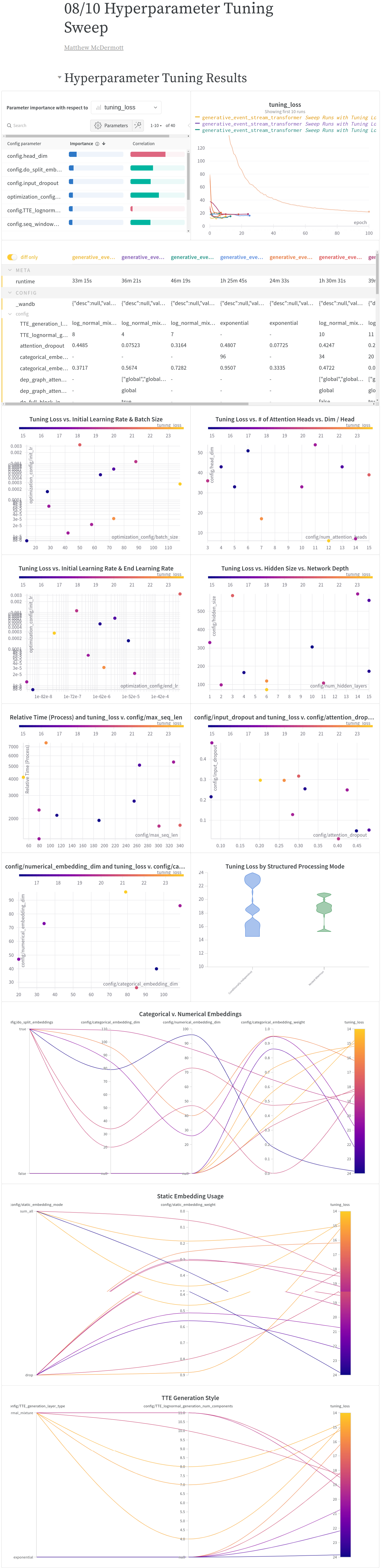Weights and biases reports for pre-training.

Evaluating Pre-trained Models¶

We provide pre-built lightning modules for assessing baseline performance on fine-tuing tasks and for running few-shot fine-tuning evaluation and zero-shot generative evaluation through user-defined labelers.

Baseline Models¶

Event Stream GPT can also aid in producing baseline performance results across both traditional, scikit-learn style models or via supervised training of ESGPT compatible neural network model architectures. For this tutorial, we build both kinds of baselines, hyperparameter tuning a random forest scikit-learn pipeline which can select between different kinds of historical aggregation windows, dimensionality reduction strategies, imputation methods, scalers, and model parameters as well as a non-pre-trained transformer model across the full parameter space therein.

The scikit-learn hyperparameter search pipeline is managed by scripts/launch_sklearn_baseline_supervised_wandb_hp_sweep.py, which leverages the Hydra config configs/sklearn_models/sklearn_baseline_hyperparameter_sweep_base.yaml. Similar to the pre-training hyperparameter tuning script, users can leverage a provided sample weights and biases template report here to track the results of this hyperparameter search. For a concrete example, in the linked report, embedded as an image below, we show that for predicting in hospital mortality on the MIMIC-IV pipeline, a random forest pipeline can achieve up to at least 0.7 AUROC in this setting.

Weights and biases reports for training a sklearn pipeline from scratch..

Additionally, users can hyperparameter tune a neural network trained from scratch on just a supervised task (for comparison against pre-trained/fine-tuned models). Such a search can be run using the scripts/launch_from_scratch_supervised_wandb_hp_sweep.py script and configs/from_scratch_supervised_hyperparameter_sweep_base.yaml config and tracked via template wandb report here. Doing so for the readmission risk prediction task on our sample MIMIC-IV pipeline shows that models can achieve peak tuning-set performance of an AUROC of 0.59.

Few-shot performance¶

To fine-tune a model, use the scripts/finetune.py script. Much like pre-training, this script leverages hydra to run, but now using the FinetuneConfig structured config object. To perform evaluation, for our working example we can run the following command:

PYTHONPATH="$EVENT_STREAM_PATH:$PYTHONPATH" \
	python $EVENT_STREAM_PATH/scripts/finetune.py \
	load_from_model_dir="$MODEL_DIR" \
	task_df_name="$TASK_NAME" \
	data_config.train_subset_size="$FT_SUBSET_SIZE" \
	data_config.train_subset_seed="$FT_SUBSET_SEED"

In this example, we ran this command for the two tasks discussed previously; 30-day readmission risk prediction and in-hospital mortality prediction, with FT_SUBSET_SIZE set to 10, 50, and 250. After running this command, the evaluation script will do the following:

1. Make a subdirectory to house model results, with the following syntax: $MODEL_DIR/finetuning/run_specifier..., where run_specifier is either $TASK_NAME for zero-shot runs (which are produced with a different script; see below) or subset_size_$FT_SUBSET_SIZE/subset_seed_$FT_SUBSET_SEED/$TASK_NAME for few-shot runs.

2. Fine-tune a model in those sub-directories, initializing from the pre-trained model’s saved weights. This model is logged to weights and biases by default (though you may need to customize the project name). Note that, by default, this model will use the same hyperparameters as the pre-trained model from which it was initialized; this is unavoidable for architectural parameters, but is likely sub-optimal for regularization parameters.

3. Upon completion, outputs its final metrics to tuning_metrics.json and held_out_metrics.json.

When fine-tuning a model, there are still some hyperparameters that can be tuned on the specific task in question, including dropout rates, batch sizes and learning rates, and weight decay parameters. We also support hyperparameter tuning over these parameters via the scripts/launch_finetuning_wandb_hp_sweep.py command, which uses the Hydra configuration file defined in configs/finetuning_hyperparameter_sweep_base.yaml to run a weights and biases sweep over only these modifiable fine-tuning parameters. Much like in pre-training and for the baseline models, there is a template report users can leverage to analyze the results of these sweeps, available here.

When we run this procedure for the Readmission Risk prediction task over MIMIC-IV, we find that fine-tuned models are able to obtain peak tuning-set performance of an AUROC of 0.61, which is slightly higher than the trained-from-scratch nueral network performance, suggesting that even on this small dataset, we do observe some benefits from generative pre-training.

Zero-shot Performance¶

Building on the existing HuggingFace API, you can also generate future values given a generative model very easily and, through this, perform zero-shot evaluation. You can use generation to perform zero-shot predictions for a given fine-tuning task by following the following steps:

1. Make a new python file which contains a “labeler”: a python object subclassing the Labeler interface which implements a __call__ method taking as input a batch of data, an input sequence length, and a configuration file and predict your task’s label. from that batch, if possible, and otherwise indicate that it is not possible. For example, if your task is to predict in-hospital mortality, your class would need to look at the elements of the batch after the input sequence length and see if any death events happen before the first discharge event.

2. You need to copy this labeling class definition file (all necessary functions and such used by the class must live in that single file) into the data directories task dataframes subfolder with the name ${task_df_name}_labeler.py.

3. You can then use the scripts/zeroshot.py script to run a zero-shot evaluation via a Hydra config on that task labeler and any pre-trained model.

For example, in this working example we provide lablers for both in-hospital mortality and readmission risk. After copying these to the data cohort task directory, we can then run the following command to perform zero-shot evaluation:

PYTHONPATH="$EVENT_STREAM_PATH:$PYTHONPATH" \
	python $EVENT_STREAM_PATH/scripts/zeroshot.py \
	load_from_model_dir="$MODEL_DIR" \
	task_df_name="$TASK_NAME" \
	config.task_specific_params.num_samples=3 data_config.do_include_start_time_min=True \
	data_config.seq_padding_side=left data_config.max_seq_len=128

This code will execute the following steps:

1. Make a subdirectory to house model results, with the following syntax: $MODEL_DIR/finetuning/$TASK_NAME.

2. Iterate over the fine-tuning dataset and generate task_specific_params.num_samples samples off of each input, then use the labeler to assess the empirical labels and probabilitiy of an input being unpredictable for these generated samples.

3. Upon completion, store final metrics to zero_shot_tuning_metrics.json and zero_shot_held_out_metrics.json.

Note that zero-shot evaluation takes a non-trivial amount of time, as generating future samples for event stream data is significantly more computationally expensive than generating traditional samples is, due to the intra-event dependencies. Much like for few-shot fine-tuning, given our small dataset size, here we again see negligible performance when running this command for the MIMIC-IV cohort and tasks. We do see, however, that only a small fraction of events are unpredictable under this approach on real world data (\(<5\%\) for mortality prediction and \(<0.5\%\) for readmission risk prediction), indicating this approach may be sufficiently robust to be used in other settings.

References¶

References

Alistair EW Johnson, Lucas Bulgarelli, Lu Shen, Alvin Gayles, Ayad Shammout, Steven Horng, Tom J Pollard, Benjamin Moody, Brian Gow, Li-wei H Lehman, and others. Mimic-iv, a freely accessible electronic health record dataset. Scientific data, 10(1):1, 2023.